Vasicek Quantile Regression in Stan

stan
quantile
Author

Sean Pinkney

Published

October 14, 2022

In this post I’ll show a way to do quantile regression on a bounded unit interval. The Vasicek distribution is an alternative distribution for beta regressions and is described in Mazucheli et al. (2022). The Vasicek distribution is given as

\[ \begin{aligned} f(y \mid \alpha, \theta) &= \sqrt{\frac{1 - \theta}{\theta}} \exp \bigg\{\frac{1}{2} \bigg[\Phi^{-1}(y)^2 - \bigg(\frac{\Phi^{-1}(y) \sqrt{1 - \theta} - \Phi^{-1}(\alpha)}{\sqrt{\theta}} \bigg)^2 \bigg\} \\ F(y \mid \alpha, \theta) &= \Phi \bigg( \frac{\Phi^{-1}(y) \sqrt{1 - \theta} - \Phi^{-1}(\alpha)}{\sqrt{\theta}} \bigg) \\ Q(\tau \mid \alpha, \theta) &= F^{-1}(\tau \mid \alpha, \theta) = \Phi \bigg( \frac{\Phi^{-1}(\alpha) + \Phi^{-1}(\tau) \sqrt{\theta}}{\sqrt{1 - \theta}} \bigg) \end{aligned} \] where \(0 < (y, \alpha, \theta, \tau) < 1\) and \(\Phi\) and \(\Phi^{-1}\) are the standard normal CDF and QF respectively. The mean of the distribution is \(\operatorname{E}(Y) = \alpha\) and \(\operatorname{Var}(Y) = \Phi_2(\Phi^{-1}(\alpha), \Phi^{-1}(\alpha), \theta)\) where \(\Phi_2\) is the bivariate standard normal CDF.

In the paper they reparameterize the mean in terms of the \(\tau\)-th quantile as \[ \alpha = h^{-1}(\mu) = \Phi(\Phi^{-1}(\mu)\sqrt{1 - \theta} - \Phi^{-1}(\tau)\sqrt{\theta}). \] Given this reparmeterization the log-likelihood is \[ \begin{aligned} \ell( \mu, \theta \mid y, \tau) = \;& \frac{n}{2}\log\bigg(\frac{1 - \theta}{\theta} \bigg) - \frac{\Phi^{-1}(y)^\top \Phi^{-1}(y)}{2} - \\ & \frac{1}{2\theta} \sum_{i=1}^{n} \bigg(\sqrt{1 - \theta}\bigg[\Phi^{-1}(y_i) - \Phi^{-1}(\mu) \bigg] + \sqrt{\theta}\Phi^{-1}(\tau) \bigg)^2 \end{aligned} \] The log-likelihood may be written in Stan as:

  real vasicek_quantile_lpdf(vector y, real theta, vector mu, real tau) {
    if (tau <= 0 || tau >= 1) 
      reject("tau must be between 0 and 1 found tau = ", tau);
    
    if (theta <= 0 || theta >= 1) 
      reject("theta must be between 0 and 1 found theta = ", theta);
    
    int N = num_elements(y);
    real lpdf = 0.5 * N * (log1m(theta) - log(theta));
    vector[N] qnorm_mu = inv_Phi(mu);
    real qnorm_tau = inv_Phi(tau);
    vector[N] qnorm_y = inv_Phi(y);
    vector[N] qnorm_alpha = -sqrt(theta) * qnorm_tau + 
                              qnorm_mu * sqrt(1 - theta);
    
    return lpdf + 0.5 * dot_self(qnorm_y) -
            0.5 * sum( (sqrt(1 - theta) * qnorm_y - qnorm_alpha)^2 / theta);
  }

The authors provided an R package vasicekreg where we can check if it results in the same log-likelihood,

library(cmdstanr)
library(vasicekreg)
source("expose_cmdstanr_funs.R")
x <- rVASIQ(n = 1, mu = 0.50, sigma = 0.69, tau = 0.50)
expose_cmdstanr_functions("vasicek.stan", expose_to_global_env = T)
stan_lpdf <- vasicek_quantile_lpdf(x, theta = 0.69, mu = 0.5, tau = 0.5)
r_lpdf <- dVASIQ(x, mu = 0.5, sigma = 0.69, log = T)
all.equal(stan_lpdf, r_lpdf)
[1] TRUE

To expose the Stan function to my R environment I have used the expose_cmdstanr_funs.R script from Rok Češnovar’s repo.

We can test this out aginst the R package fit. The following Stan code performs the regression.

Now, let’s see how the package and Stan compare.

set.seed(123)
n <- 100
x <- rbinom(n, size = 1, prob = 0.5)
eta <- 0.5 + 1 * x;
mu <- 1 / (1 + exp(-eta));
sigma <- 0.5;
y <- rVASIQ(n, mu, sigma, tau = 0.5)
data <- data.frame(y, x, tau = 0.5)
tau <- 0.5;
fit_gamlss <- gamlss::gamlss(y ~ x, data = data, family = VASIQ)
GAMLSS-RS iteration 1: Global Deviance = -55.4043 
GAMLSS-RS iteration 2: Global Deviance = -55.4042 
summary(fit_gamlss)
******************************************************************
Family:  c("VASIQ", "VasicekQ") 

Call:  gamlss::gamlss(formula = y ~ x, family = VASIQ, data = data) 

Fitting method: RS() 

------------------------------------------------------------------
Mu link function:  logit
Mu Coefficients:
            Estimate Std. Error t value Pr(>|t|)   
(Intercept)   0.6554     0.1936   3.385  0.00103 **
x             0.9284     0.2975   3.120  0.00238 **
---
Signif. codes:  0 '***' 0.001 '**' 0.01 '*' 0.05 '.' 0.1 ' ' 1

------------------------------------------------------------------
Sigma link function:  logit
Sigma Coefficients:
            Estimate Std. Error t value Pr(>|t|)  
(Intercept)  -0.2929     0.1414  -2.071    0.041 *
---
Signif. codes:  0 '***' 0.001 '**' 0.01 '*' 0.05 '.' 0.1 ' ' 1

------------------------------------------------------------------
No. of observations in the fit:  100 
Degrees of Freedom for the fit:  3
      Residual Deg. of Freedom:  97 
                      at cycle:  2 
 
Global Deviance:     -55.40424 
            AIC:     -49.40424 
            SBC:     -41.58873 
******************************************************************
mod <- cmdstan_model("vasicek.stan")
fit_stan <- mod$sample(
  data = list(N = n,
              y = y,
              x = x,
              tau = 0.5),
  refresh = 0,
  show_messages = FALSE,
  parallel_chains = 4
)
Running MCMC with 4 parallel chains...

Chain 1 finished in 0.1 seconds.
Chain 2 finished in 0.1 seconds.
Chain 3 finished in 0.1 seconds.
Chain 4 finished in 0.2 seconds.

All 4 chains finished successfully.
Mean chain execution time: 0.1 seconds.
Total execution time: 0.3 seconds.
fit_stan$summary()
# A tibble: 4 × 10
  variable   mean median    sd   mad     q5     q95  rhat ess_bulk ess_tail
  <chr>     <dbl>  <dbl> <dbl> <dbl>  <dbl>   <dbl> <dbl>    <dbl>    <dbl>
1 lp__     26.2   26.5   1.18  0.957 23.9   27.5     1.00    1981.    2224.
2 alpha     0.657  0.654 0.198 0.199  0.330  0.985   1.00    2456.    2752.
3 beta      0.936  0.931 0.296 0.302  0.445  1.42    1.00    2470.    2200.
4 sigma    -0.263 -0.268 0.141 0.141 -0.483 -0.0209  1.00    2616.    2473.

Similar results!

We can update the code to run multiple quantiles which is the same as running the model for each quantile. In Stan, we can run the same model multiple times or we do the loop, as I show below, inside the program and pass a vector of \(\tau\)’s in as data.

fittaus <- lapply(c(0.10, 0.25, 0.50, 0.75, 0.90), function(Tau)
 {
  tau <<- Tau; 
  gamlss::gamlss(y ~ x, data = data, family = VASIQ)
 })

gamlss_mtau <-  sapply(fittaus, function(x) summary(x)[, 1])


mod_vector <- cmdstan_model("vasciek_vector_tau.stan")
fit_stan_vector <- mod_vector$sample(
  data = list(N = n,
              y = y,
              x = x,
              K = 5,
              tau = c(0.1,0.25, 0.5, 0.75, 0.9)),
  refresh = 0,
  show_messages = FALSE,
  parallel_chains = 4
)

The parameter results

data.frame(stan = fit_stan_vector$summary()[-1, 1:2], 
           gamlss_estimates =c(t(gamlss_mtau)))
   stan.variable  stan.mean gamlss_estimates
1       alpha[1] -1.1768928       -1.1439249
2       alpha[2] -0.2992555       -0.2798790
3       alpha[3]  0.6571251        0.6553778
4       alpha[4]  1.6818706        1.6508267
5       alpha[5]  2.7209694        2.6706897
6        beta[1]  0.8880346        0.8953157
7        beta[2]  0.8795350        0.8746433
8        beta[3]  0.9316846        0.9284407
9        beta[4]  1.0657726        1.0609815
10       beta[5]  1.2600745        1.2410836
11      sigma[1] -0.2602243       -0.2913405
12      sigma[2] -0.2638038       -0.2927525
13      sigma[3] -0.2616609       -0.2928563
14      sigma[4] -0.2575334       -0.2927568
15      sigma[5] -0.2588908       -0.2914669

Aki Veharti correctly noted that the increase in the number of parameters will reduce the step size and increase the number of steps. If you have lots of data then it may make more sense to run each \(\tau\) independently.

individual_fit <- fit_stan$sampler_diagnostics()[,,c("stepsize__", 
                                                     "n_leapfrog__")]
vector_fit <- fit_stan_vector$sampler_diagnostics()[,,c("stepsize__",
                                                        "n_leapfrog__")]

data.frame(stepsize_avg = round(c(mean(individual_fit[, , 1]),
                                  mean(vector_fit[, , 1])), 2),
           n_leapfrog_avg = round(c(mean(individual_fit[, , 2]), 
                                    mean(vector_fit[, , 2])), 2),
           row.names = c("individual_fit", "vector_fit"))
               stepsize_avg n_leapfrog_avg
individual_fit         0.57           5.84
vector_fit             0.38          13.10

We see that the sampler must take smaller steps and increase the number of leapfrog integrations.

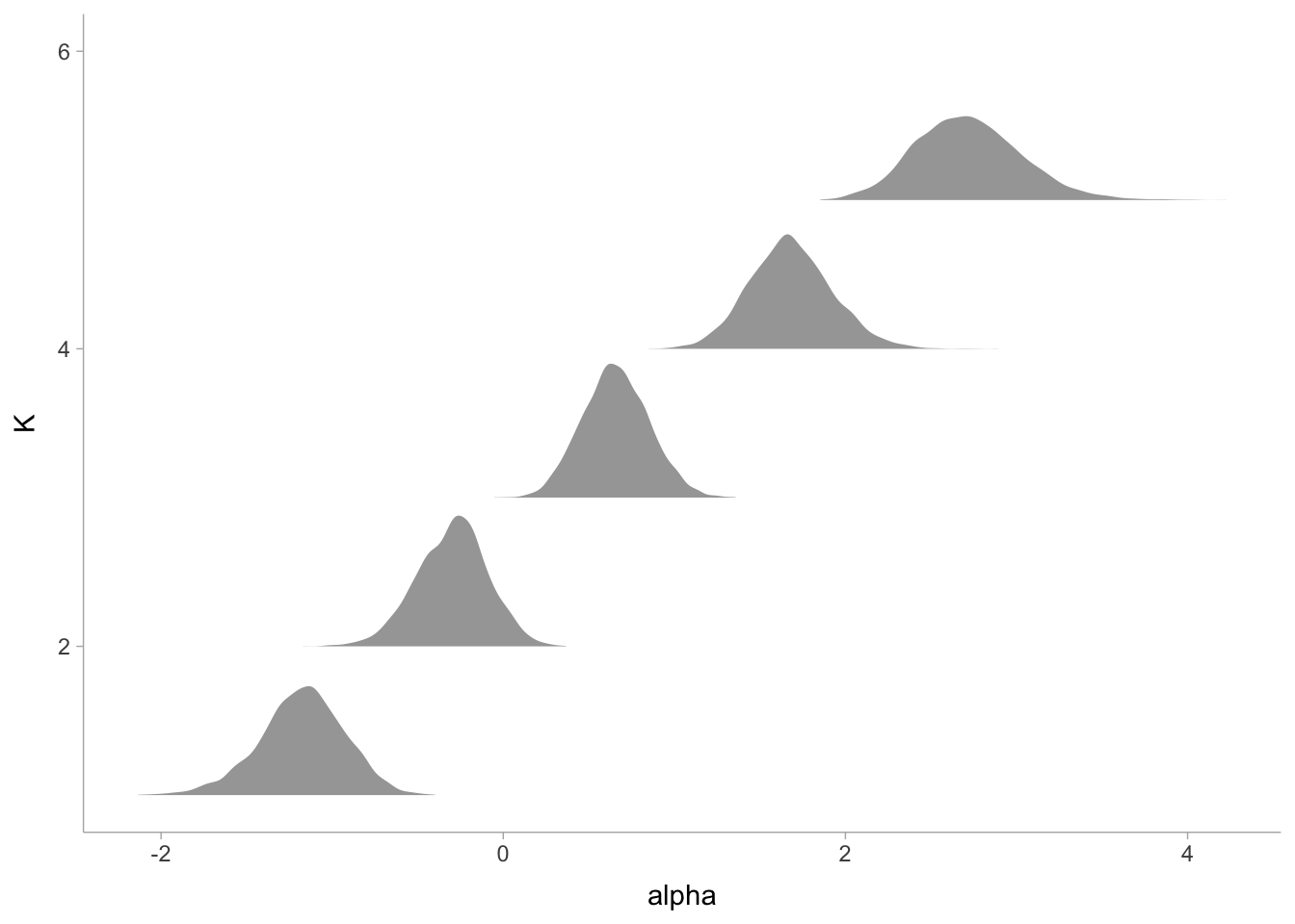
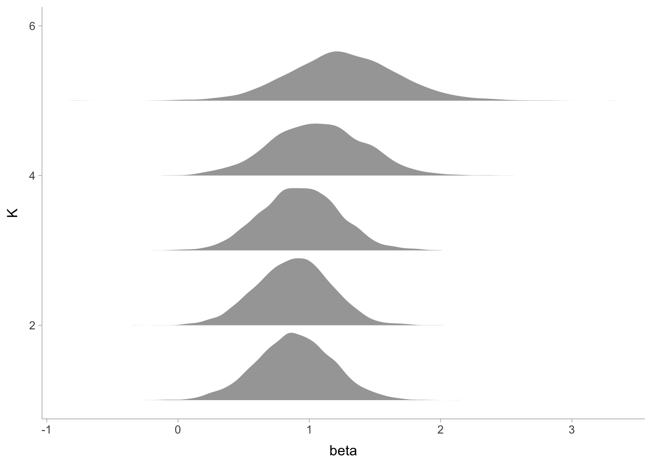
Lastly, we can plot the effects. Here are the intercepts and beta coefficients

library(posterior)
library(tidybayes)
library(ggplot2)
theme_set(theme_tidybayes())

fit_stan_vector |>
  spread_draws(alpha[K]) |>
  ggplot(aes(y = K, x = alpha))  +
  stat_slabh()

fit_stan_vector |>
  spread_draws(beta[K]) |>
  ggplot(aes(y = K, x = beta))  +
  stat_slabh()

In my next post, quantile regression post I’ll show various ways to represent a quantile regression in Stan where the outcome, however, is continuous on the real line.

Appendix

Single tau

functions {
  real vasicek_quantile_lpdf(vector y, real theta, vector mu, real tau) {
    int N = num_elements(y);
    real lpdf = 0.5 * N * (log1m(theta) - log(theta));
    vector[N] qnorm_mu = inv_Phi(mu);
    real qnorm_tau = inv_Phi(tau);
    vector[N] qnorm_y = inv_Phi(y);
    vector[N] qnorm_alpha = -sqrt(theta) * qnorm_tau + 
                              qnorm_mu * sqrt(1 - theta);
    
    return lpdf + 0.5 * dot_self(qnorm_y) - 
            0.5 * sum( (sqrt(1 - theta) * qnorm_y - qnorm_alpha)^2 / theta);
  }
}
data {
  int<lower=0> N;
  vector[N] y;
  vector[N] x;
  real<lower=0, upper=1> tau;
} 
parameters {
  real alpha;
  real beta;
  real sigma;
} 
model {
  alpha ~ normal(0, 4);
  beta ~ normal(0, 4);
  sigma ~ normal(0, 2);
  y ~ vasicek_quantile(inv_logit(sigma), inv_logit(alpha + beta * x), tau);
}

Multiple tau

functions {
  real vasicek_quantile_lpdf(vector y, real theta, vector mu, real tau) {
    if (tau <= 0 || tau >= 1) 
      reject("tau must be between 0 and 1 found tau = ", tau);
    
    if (theta <= 0 || theta >= 1) 
      reject("theta must be between 0 and 1 found theta = ", theta);
    
    int N = num_elements(y);
    real lpdf = 0.5 * N * (log1m(theta) - log(theta));
    vector[N] qnorm_mu = inv_Phi(mu);
    real qnorm_tau = inv_Phi(tau);
    vector[N] qnorm_y = inv_Phi(y);
    vector[N] qnorm_alpha = -sqrt(theta) * qnorm_tau +  
                              qnorm_mu * sqrt(1 - theta);
    
    return lpdf + 
            0.5 * dot_self(qnorm_y) - 
            0.5 * sum( (sqrt(1 - theta) * qnorm_y - qnorm_alpha)^2 / theta);
  }
}
data {
  int<lower=0> N;
  vector[N] y;
  vector[N] x;
  
  int<lower=1> K;
  vector<lower=0, upper=1>[K] tau;
} 
parameters {
  vector[K] alpha;
  vector[K] beta;
  vector[K] sigma;
} 
model {
  alpha ~ normal(0, 4);
  beta ~ normal(0, 4);
  sigma ~ normal(0, 2);
  
  for (i in 1:K)
    y ~ vasicek_quantile(inv_logit(sigma[i]), 
                         inv_logit(alpha[i] + beta[i] * x), tau[i]);
}

References

Mazucheli, Josmar, Bruna Alves, Mustafa Ç. Korkmaz, and Víctor Leiva. 2022. “Vasicek Quantile and Mean Regression Models for Bounded Data: New Formulation, Mathematical Derivations, and Numerical Applications.” Mathematics 10 (9). https://doi.org/10.3390/math10091389.