Quantile regressions are relatively new in the Bayesian literature first appearing in Yu and Moyeed (2001) who described an asymmetric Laplace distribution to estimate the conditional quantiles. This post is going to show the asymmetric Laplace and the augmented version. In part II I will show the score likelihood method.
The asymmetric Laplace distribution is given as \[ \operatorname{ALD}(Y \mid x, \beta) = \frac{\tau^n (1 - \tau)^n}{\sigma^n}\exp \bigg( -\frac{\sum_{i=1}^n \rho_\tau (y_i - x_i^{\top}\beta)}{\sigma} \bigg) \]
where
\[ \rho_\tau(u) = \frac{|u| + (2\tau - 1)u}{2} \]
We may write this in Stan as
functions{
real q_loss(real q, vector u){
  return 0.5 * sum(abs(u) + (2 * q - 1) * u);
}

real ald_lpdf(vector y, real q, real sigma, vector q_est){
  int N = num_elements(y);

  return N * (log(q) + log1m(q) - log(sigma)) - q_loss(q, y - q_est) / sigma;
}
}
data {
  int N;                   // Number of observation
  int P;                   // Number of predictors
  real<lower=0, upper=1> q;
  vector[N] y;             // Response variable sorted
  matrix[N, P] x;
}
parameters {
  vector[P] beta;
  real<lower=0> sigma;
}
model {
  beta ~ normal(0, 4);
  sigma ~ exponential(1);
  y ~ ald(q, sigma, x * beta);
}
Let’s compare the 5th percentile to the Brq R package
library(Brq)
data("ImmunogG")
out_asym_laplace <- asymetric_laplace$sample(
  data = list(N = nrow(ImmunogG),
              P = 3,
              q = 0.05,
              y = ImmunogG$IgG,
              x = as.matrix(data.frame(alpha = 1, x = ImmunogG$Age, xsq = ImmunogG$Age^2))),
  seed = 12123123,
  parallel_chains = 4,
  iter_warmup = 500,
  iter_sampling = 500,
    refresh = 0,
  show_messages = FALSE
)
Running MCMC with 4 parallel chains...
Chain 1 finished in 0.5 seconds.
Chain 3 finished in 0.4 seconds.
Chain 4 finished in 0.5 seconds.
Chain 2 finished in 0.6 seconds.
All 4 chains finished successfully.
Mean chain execution time: 0.5 seconds.
Total execution time: 0.7 seconds.out_asym_laplace$summary()# A tibble: 5 × 10
variable mean median sd mad q5 q95 rhat ess_bulk
<chr> <dbl> <dbl> <dbl> <dbl> <dbl> <dbl> <dbl> <dbl>
1 lp__ -670. -670. 1.50 1.24 -673. -669. 1.01 585.
2 beta[1] 0.587 0.601 0.246 0.271 0.179 0.962 1.02 385.
3 beta[2] 1.31 1.31 0.199 0.210 1.01 1.64 1.02 336.
4 beta[3] -0.156 -0.155 0.0338 0.0333 -0.212 -0.104 1.01 373.
5 sigma 0.165 0.165 0.00958 0.00897 0.149 0.181 1.01 645.
# … with 1 more variable: ess_tail <dbl>y = ImmunogG$IgG
x = ImmunogG$Age
X=cbind(x, x^2)
fit = Brq(y ~ X , tau= 0.05,runs= 2000, burn=1000)
print(summary(fit))Call:
Brq.formula(formula = y ~ X, tau = 0.05, runs = 2000, burn = 1000)
tau:[1] 0.05
Estimate L.CredIntv U.CredIntv
Intercept 0.6285948 0.1193195 1.04185440
Xx 1.2928087 0.8984968 1.67267316
X -0.1541316 -0.2265564 -0.08528427Scale-mixture representation
The above may also be written as a mixture of exponential and normal distributions. Letting
\[ \begin{aligned} z_i &\sim \operatorname{Exp}(1) \\ \sigma &\sim \operatorname{Exp}(1) \\ y_i &\sim \mathcal{N}(x_i^{\top}\beta_p + \sigma \theta z_i,\, \tau \sigma \sqrt{z_i}) \end{aligned} \] where
\[ \begin{aligned} \theta &= \frac{1 - 2 q}{q (1 - q)} \\ \tau &= \sqrt{\frac{2}{q(1 -q)}} \end{aligned} \]
The following Stan model implements the augmented approach.
data {
  int N;                   // Number of observation
  int P;                   // Number of predictors
  real<lower=0, upper=1> q;
  vector[N] y;             // Response variable sorted
  matrix[N, P] x;
}
transformed data {
  real theta = (1 - 2 * q) / (q * (1 - q));
  real tau = sqrt(2 / (q * (1 - q)));
}
parameters {
  vector[P] beta;
  vector<lower=0>[N] z;
  real<lower=0> sigma;
}
model {
  beta ~ normal(0, 2);
  sigma ~ exponential(1);

  // Data Augmentation
  z ~ exponential(1);
  y ~ normal(x * beta + sigma * theta * z, tau * sqrt(z) * sigma);
}
Let’s fit the model
out_aug_laplace <- augmented_laplace$sample(
  data = list(N = nrow(ImmunogG),
              P = 3,
              q = 0.05,
              y = ImmunogG$IgG,
              x = as.matrix(data.frame(alpha = 1, x = ImmunogG$Age, xsq = ImmunogG$Age^2))),
  seed = 12123123,
  parallel_chains = 4,
  iter_warmup = 500,
  iter_sampling = 500,
    refresh = 0,
  show_messages = FALSE
)
Running MCMC with 4 parallel chains...
Chain 1 finished in 3.7 seconds.
Chain 3 finished in 3.7 seconds.
Chain 2 finished in 4.0 seconds.
Chain 4 finished in 4.1 seconds.
All 4 chains finished successfully.
Mean chain execution time: 3.9 seconds.
Total execution time: 4.2 seconds.Warning: 77 of 2000 (4.0%) transitions ended with a divergence.
See https://mc-stan.org/misc/warnings for details.out_aug_laplace$summary("beta")# A tibble: 3 × 10
variable mean median sd mad q5 q95 rhat ess_bulk ess_tail
<chr> <dbl> <dbl> <dbl> <dbl> <dbl> <dbl> <dbl> <dbl> <dbl>
1 beta[1] 0.589 0.596 0.249 0.264 0.169 0.982 1.01 443. 733.
2 beta[2] 1.31 1.32 0.210 0.201 0.953 1.64 1.01 397. 505.
3 beta[3] -0.155 -0.155 0.0354 0.0321 -0.216 -0.0973 1.01 394. 522.Ouch! Divergences. Although the parameter estimates look comparable. Let’s inspect the pairs plots between the augmented version and the asymmetric Laplace.
library(bayesplot)This is bayesplot version 1.9.0- Online documentation and vignettes at mc-stan.org/bayesplot- bayesplot theme set to bayesplot::theme_default() * Does _not_ affect other ggplot2 plots * See ?bayesplot_theme_set for details on theme settingnp_aug_laplace <- nuts_params(out_aug_laplace)
np_asym_laplace <- nuts_params(out_asym_laplace)
mcmc_pairs(out_aug_laplace$draws(c("beta", "sigma")), np = np_aug_laplace)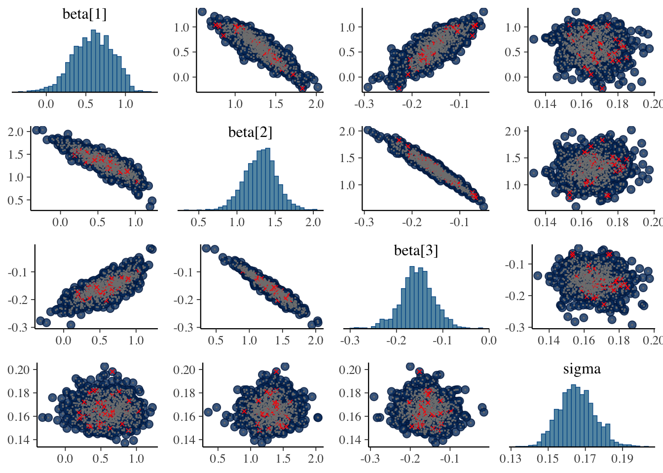
mcmc_pairs(out_asym_laplace$draws(c("beta", "sigma")), np = np_asym_laplace)
The pairs plots don’t appear to show the divergence originating be due to beta or sigma. It’s most likely the augmentation variables z. As I’m up for time on this, I’d be curious to test out alternative specifications or see if anyone has encountered these issues with the augmented version and found a solution.
For the next post, we’ll take a look at an approximate likelihood using the data which asymptotically approaches the true likelihood with more data.