Latent Class Analysis on a Restricted Poincaré Disk

Geometry-Based Identification with BLAS-Accelerated Likelihood

stan
model
Author

Sean Pinkney

Published

February 28, 2026

Show the code
import numpy as np
import pandas as pd
import logging
from collections import Counter
from scipy.special import expit as sigmoid
from cmdstanpy import CmdStanModel
import matplotlib.pyplot as plt
import matplotlib.gridspec as gridspec
from matplotlib.colors import LinearSegmentedColormap
import subprocess
import textwrap
import shutil

# Silence CmdStanPy INFO logs in rendered output.
logging.getLogger("cmdstanpy").setLevel(logging.WARNING)
logging.getLogger("cmdstanpy").propagate = False

np.random.seed(42)
blog = {
    "background": "#f0f2f5",
    "text": "#24292e",
    "text_light": "#6a737d",
    "teal": "#0d7d6c",
    "blue": "#0366d6",
    "purple": "#6f42c1",
    "gold": "#b08800",
    "red": "#cb2431",
    "navy": "#032f62",
    "grid": "#e1e4e8",
}
colors = [blog["teal"], blog["blue"], blog["purple"], blog["gold"], blog["red"], blog["navy"]]

plt.rcParams.update({
    "figure.facecolor": blog["background"],
    "axes.facecolor": blog["background"],
    "axes.edgecolor": blog["text_light"],
    "axes.labelcolor": blog["text"],
    "axes.titlecolor": blog["text"],
    "text.color": blog["text"],
    "xtick.color": blog["text_light"],
    "ytick.color": blog["text_light"],
    "grid.color": blog["grid"],
    "grid.linestyle": "-",
    "grid.linewidth": 0.6,
    "axes.grid": True,
    "legend.facecolor": blog["background"],
    "legend.edgecolor": blog["grid"],
})

def style_axes(ax, grid=True):
    ax.set_facecolor(blog["background"])
    if grid:
        ax.grid(True, color=blog["grid"], linewidth=0.6, alpha=0.9)
    else:
        ax.grid(False)
    for spine in ax.spines.values():
        spine.set_color(blog["text_light"])
        spine.set_linewidth(0.8)

1. Why This Model

This post fits a 3-class latent class model where each class is a point on a restricted Poincare disk. The geometry gives a direct interpretation of class differences, and an ordering constraint on radii gives identification without post-hoc relabeling.

The goals are:

  1. Fit an identified Bayesian LCA with interpretable latent coordinates.
  2. Use a fast collapsed likelihood on sufficient statistics.
  3. Verify that the geometric model recovers clear class separation.
  4. Compare the fitted profiles to a standard poLCA baseline.

2. Data

I use the synthetic drinking-behavior data from the UCLA OARC LCA tutorial (UCLA Statistical Consulting Group 2026). The dataset has \(N = 1{,}000\) respondents and \(J = 9\) binary items:

Item Description
j1 I like to drink
j2 I drink hard liquor
j3 I have drank in the morning
j4 I have drank at work
j5 I drink to get drunk
j6 I like the taste of alcohol
j7 I drink to help me sleep
j8 Drinking interferes with my relationships
j9 I frequently visit bars
Show the code
item_labels = [
    "Like to drink", "Hard liquor", "Morning drinking",
    "Drinking at work", "Drink to get drunk", "Like taste",
    "Drink to sleep", "Interferes w/ relationships", "Visit bars"
]

raw = np.loadtxt("data/lca1.csv", delimiter=",", dtype=int)
Y = raw[:, 1:]  # drop row ID
N, J = Y.shape
print(f"N = {N}, J = {J}")
N = 1000, J = 9

2.1 Descriptive Statistics

Show the code
means = Y.mean(axis=0)
desc = pd.DataFrame({
    "Item": [f"j{j+1}" for j in range(J)],
    "Description": item_labels,
    "Endorsement Rate": [f"{m:.1%}" for m in means]
})
desc
Item Description Endorsement Rate
0 j1 Like to drink 69.3%
1 j2 Hard liquor 29.1%
2 j3 Morning drinking 8.3%
3 j4 Drinking at work 9.0%
4 j5 Drink to get drunk 19.9%
5 j6 Like taste 28.2%
6 j7 Drink to sleep 13.9%
7 j8 Interferes w/ relationships 16.7%
8 j9 Visit bars 27.7%

Endorsement rates range from under 10% (morning drinking, drinking at work) to almost 70% (liking to drink). So the item set spans lower-risk and higher-risk behavior.

2.2 Sufficient Statistics

For computational speed, I collapse the \(N=1{,}000\) response vectors into \(P\) unique patterns with counts. This keeps the likelihood exact but avoids repeated evaluations of identical rows:

Show the code
patterns = [tuple(row) for row in Y]
counts = Counter(patterns)
unique = sorted(counts.keys())
pat = np.array(unique, dtype=int)
cnt = np.array([counts[p] for p in unique], dtype=int)
P = pat.shape[0]
print(f"{N} observations → {P} unique patterns")
print(f"Most common: {cnt.max()} occurrences, {(cnt == 1).sum()} singletons")
1000 observations → 180 unique patterns
Most common: 126 occurrences, 87 singletons

3. Model

3.1 Identification Problem

Finite mixtures have label symmetry: with \(K\) classes there are \(K!\) equivalent posterior modes (Stephens 2000; Jasra, Holmes, and Stephens 2005). Without identifying structure, MCMC can jump across class permutations and make class summaries hard to interpret.

I use a geometric identification strategy: classes are embedded on a restricted Poincare disk (Nickel and Kiela 2017), and class labels are fixed by ordering radii.

3.2 Geometric Class Coordinates

Each class is a point on the open unit disk with polar coordinates \((r_k,\alpha_k)\), where \(r_k\in(0,1)\) and \(\alpha_k\in(0,\pi/2)\). Item directions are fixed and evenly spaced: \[ \varphi_j = \frac{\pi}{2} \cdot \frac{j-1}{J-1}, \qquad j = 1, \ldots, J \] so all items lie in the same quadrant.

3.3 Item-Response Probabilities

The class-\(k\) endorsement probability for item \(j\) is \[ \theta_{kj} = \text{logit}^{-1}\!\Big(\alpha_j + \lambda_j \, r_k \cos(\alpha_k - \varphi_j)\Big) \] where:

  • \(\alpha_j \in \mathbb{R}\) is the item baseline,
  • \(\lambda_j > 0\) is item discrimination,
  • \(r_k \cos(\alpha_k - \varphi_j)\) is the projection of class position onto item direction.

Because both angles are restricted to \([0,\pi/2]\), we have \(\cos(\alpha_k-\varphi_j)\ge 0\). Increasing radius therefore cannot lower an item below its baseline \(\text{logit}^{-1}(\alpha_j)\), which removes one common source of multimodality.

The two coordinates have a direct interpretation:

  • Radius \(r_k\): global severity (closer to 1 means higher overall propensity to endorse).
  • Angle \(\alpha_k\): profile direction (which subset of items gets the strongest lift).

3.4 Mixture Likelihood and Ordering Constraint

The collapsed-pattern likelihood is: \[ p(\mathbf{y}_p) = \sum_{k=1}^K \pi_k \prod_{j=1}^J \theta_{kj}^{y_{pj}} (1 - \theta_{kj})^{1 - y_{pj}} \]

I break label symmetry with ordered radii: \[ \text{logit}(r_1) < \text{logit}(r_2) < \cdots < \text{logit}(r_K) \] implemented using Stan’s ordered[K] type (Carpenter et al. 2017). Class 1 is always most central and class \(K\) is always most extreme.

3.5 BLAS-Accelerated Likelihood Evaluation

For each class, the Bernoulli log-probability for pattern \(\mathbf{y}_p\) can be written as: \[ \log p(\mathbf{y}_p \mid k) = \mathbf{y}_p^\top \boldsymbol{\eta}_k - \sum_{j=1}^J \log(1 + e^{\eta_{kj}}) \] where \(\eta_{kj} = \alpha_j + \lambda_j r_k \cos(\alpha_k - \varphi_j)\). This gives a fast three-step computation:

  1. Precompute class offsets (once per leapfrog step): \[ c_k = -\sum_{j=1}^J \log(1 + e^{\eta_{kj}}) \]

  2. Single BLAS matrix multiply (\(O(PJK)\)): \[ \mathbf{S} = \mathbf{Y}\,\boldsymbol{\eta}^\top \qquad (P \times K) \]

  3. Pattern-wise log-sum-exp: \[ \text{target} \mathrel{+}= \sum_{p=1}^P n_p \log\!\sum_{k=1}^K \exp\!\big(\log \pi_k + S_{pk} + c_k\big) \]

The key speed gain comes from replacing the inner item loop with one dgemm call for \(\mathbf{Y}\eta^\top\).

3.6 Priors

Parameter Prior Notes
\(\text{logit}(r_k)\) \(\mathcal{N}(0, 2)\) Ordered in Stan for identification
\(\alpha_k^{\text{raw}}\) \(\mathcal{N}(0, 2)\) Mapped to \((0, \pi/2)\) via \((\pi/2)\,\sigma(\cdot)\)
\(\alpha_j\) \(\mathcal{N}(0, 3)\) Weakly informative item baselines
\(\lambda_j\) \(\mathcal{N}^+(0, 3)\) Half-normal via <lower=0>
\(\boldsymbol{\pi}\) \(\text{Dir}(2, \ldots, 2)\) Mild regularization toward balanced class weights

4. Inference

4.1 Compile and Optimize

I use a two-stage workflow: first multi-start optimization to locate a good mode, then NUTS initialized near that mode.

Show the code
K = 3
model = CmdStanModel(stan_file="lca_poincare.stan")
Show the code
def random_init(K, J, rng):
    logit_r = np.sort(rng.randn(K) * 0.8)
    angle_raw = rng.randn(K) * 1.0
    alpha = rng.randn(J) * 0.5
    lam = np.abs(rng.randn(J)) + 0.5
    pi_w = rng.dirichlet(np.ones(K) * 2.0)
    return dict(logit_r=logit_r.tolist(), angle_raw=angle_raw.tolist(),
                alpha=alpha.tolist(), lam=lam.tolist(), pi_w=pi_w.tolist())

def find_best_optimum(model, stan_data, n_starts=20, seed=42):
    best_opt, best_lp = None, -np.inf
    rng = np.random.RandomState(seed)
    K, J = stan_data['K'], stan_data['J']
    for i in range(n_starts):
        init = random_init(K, J, rng)
        try:
            opt = model.optimize(data=stan_data, inits=init, jacobian=True,
                                 seed=seed + i, show_console=False)
            lp = opt.optimized_params_dict['lp__']
            if lp > best_lp:
                best_lp, best_opt = lp, opt
        except Exception:
            pass
    return best_opt

def opt_to_nuts_init(opt, K, J, jitter=0.02, rng=None):
    if rng is None:
        rng = np.random.RandomState()
    d = opt.optimized_params_dict
    logit_r = np.sort(np.array([d[f'logit_r[{k+1}]'] for k in range(K)]) + rng.randn(K) * jitter)
    angle_raw = np.array([d[f'angle_raw[{k+1}]'] for k in range(K)]) + rng.randn(K) * jitter
    alpha = np.array([d[f'alpha[{j+1}]'] for j in range(J)]) + rng.randn(J) * jitter
    lam = np.maximum(np.array([d[f'lam[{j+1}]'] for j in range(J)]) + rng.randn(J) * jitter, 0.01)
    pi_w = np.maximum(np.array([d[f'pi_w[{k+1}]'] for k in range(K)]) + rng.randn(K) * jitter * 0.1, 0.01)
    pi_w /= pi_w.sum()
    return dict(logit_r=logit_r.tolist(), angle_raw=angle_raw.tolist(),
                alpha=alpha.tolist(), lam=lam.tolist(), pi_w=pi_w.tolist())
Show the code
stan_data = {'P': P, 'K': K, 'J': J, 'pattern': pat.tolist(), 'count': cnt.tolist()}

best_opt = find_best_optimum(model, stan_data, n_starts=20, seed=42)
d = best_opt.optimized_params_dict
print(f"Best lp__: {d['lp__']:.2f}")

# MAP estimates
print(f"\nMAP θ[k,j]:")
header = "         " + "".join(f"{'j'+str(j+1):>6}" for j in range(J))
print(header)
for k in range(K):
    theta_row = [sigmoid(d[f'logit_theta[{k+1},{j+1}]']) for j in range(J)]
    pi_k = d[f'pi_w[{k+1}]']
    print(f"    C{k+1}: " + "".join(f"{t:>6.2f}" for t in theta_row) + f"  π={pi_k:.3f}")
10:19:33 - cmdstanpy - INFO - Chain [1] start processing
10:19:33 - cmdstanpy - INFO - Chain [1] done processing
10:19:33 - cmdstanpy - INFO - Chain [1] start processing
10:19:33 - cmdstanpy - INFO - Chain [1] done processing
10:19:33 - cmdstanpy - INFO - Chain [1] start processing
10:19:33 - cmdstanpy - INFO - Chain [1] done processing
10:19:33 - cmdstanpy - INFO - Chain [1] start processing
10:19:33 - cmdstanpy - INFO - Chain [1] done processing
10:19:33 - cmdstanpy - INFO - Chain [1] start processing
10:19:33 - cmdstanpy - INFO - Chain [1] done processing
10:19:33 - cmdstanpy - INFO - Chain [1] start processing
10:19:33 - cmdstanpy - INFO - Chain [1] done processing
10:19:33 - cmdstanpy - INFO - Chain [1] start processing
10:19:33 - cmdstanpy - INFO - Chain [1] done processing
10:19:33 - cmdstanpy - INFO - Chain [1] start processing
10:19:33 - cmdstanpy - INFO - Chain [1] done processing
10:19:33 - cmdstanpy - INFO - Chain [1] start processing
10:19:33 - cmdstanpy - INFO - Chain [1] done processing
10:19:33 - cmdstanpy - INFO - Chain [1] start processing
10:19:33 - cmdstanpy - INFO - Chain [1] done processing
10:19:33 - cmdstanpy - INFO - Chain [1] start processing
10:19:33 - cmdstanpy - INFO - Chain [1] done processing
10:19:33 - cmdstanpy - INFO - Chain [1] start processing
10:19:33 - cmdstanpy - INFO - Chain [1] done processing
10:19:33 - cmdstanpy - INFO - Chain [1] start processing
10:19:33 - cmdstanpy - INFO - Chain [1] done processing
10:19:33 - cmdstanpy - INFO - Chain [1] start processing
10:19:33 - cmdstanpy - INFO - Chain [1] done processing
10:19:33 - cmdstanpy - INFO - Chain [1] start processing
10:19:33 - cmdstanpy - INFO - Chain [1] done processing
10:19:33 - cmdstanpy - INFO - Chain [1] start processing
10:19:33 - cmdstanpy - INFO - Chain [1] done processing
10:19:33 - cmdstanpy - INFO - Chain [1] start processing
10:19:33 - cmdstanpy - INFO - Chain [1] done processing
10:19:33 - cmdstanpy - INFO - Chain [1] start processing
10:19:33 - cmdstanpy - INFO - Chain [1] done processing
10:19:33 - cmdstanpy - INFO - Chain [1] start processing
10:19:33 - cmdstanpy - INFO - Chain [1] done processing
10:19:33 - cmdstanpy - INFO - Chain [1] start processing
10:19:33 - cmdstanpy - INFO - Chain [1] done processing
Best lp__: -4246.63

MAP θ[k,j]:
             j1    j2    j3    j4    j5    j6    j7    j8    j9
    C1:   0.49  0.17  0.02  0.04  0.07  0.22  0.08  0.10  0.26  π=0.483
    C2:   0.87  0.37  0.10  0.10  0.24  0.31  0.14  0.16  0.28  π=0.441
    C3:   0.96  0.58  0.37  0.36  0.81  0.54  0.49  0.61  0.43  π=0.076

4.2 NUTS Sampling

Show the code
chains = 4
inits = [opt_to_nuts_init(best_opt, K, J, jitter=0.02 + 0.01*c,
                           rng=np.random.RandomState(42 + c + 100))
         for c in range(chains)]

fit = model.sample(
    data=stan_data, chains=chains,
    iter_warmup=2000, iter_sampling=2000,
    seed=42, inits=inits,
    adapt_delta=0.95, max_treedepth=10,
    show_progress=False,
)
10:19:33 - cmdstanpy - INFO - CmdStan start processing
10:19:33 - cmdstanpy - INFO - Chain [1] start processing
10:19:33 - cmdstanpy - INFO - Chain [2] start processing
10:19:33 - cmdstanpy - INFO - Chain [3] start processing
10:19:33 - cmdstanpy - INFO - Chain [4] start processing
10:19:52 - cmdstanpy - INFO - Chain [1] done processing
10:19:53 - cmdstanpy - INFO - Chain [4] done processing
10:19:53 - cmdstanpy - INFO - Chain [2] done processing
10:19:54 - cmdstanpy - INFO - Chain [3] done processing

4.3 Diagnostics

Show the code
diag = fit.diagnose()
for line in diag.split('\n'):
    if line.strip():
        print(line)
Checking sampler transitions treedepth.
Treedepth satisfactory for all transitions.
Checking sampler transitions for divergences.
No divergent transitions found.
Checking E-BFMI - sampler transitions HMC potential energy.
E-BFMI satisfactory.
Rank-normalized split effective sample size satisfactory for all parameters.
Rank-normalized split R-hat values satisfactory for all parameters.
Processing complete, no problems detected.
Show the code
summary = fit.summary()
targets = ([f'logit_r[{k}]' for k in range(1, K+1)]
         + [f'angle_raw[{k}]' for k in range(1, K+1)]
         + [f'alpha[{j}]' for j in range(1, J+1)]
         + [f'lam[{j}]' for j in range(1, J+1)]
         + [f'pi_w[{k}]' for k in range(1, K+1)])

conv_rows = []
for p in targets:
    if p in summary.index:
        row = summary.loc[p]
        rhat = row.get('R_hat', row.get('Rhat', float('nan')))
        ess = row.get('N_Eff', row.get('ESS_bulk', float('nan')))
        conv_rows.append({"Parameter": p, "R-hat": f"{rhat:.3f}", "ESS": f"{ess:.0f}"})

pd.DataFrame(conv_rows)
Parameter R-hat ESS
0 logit_r[1] 1.001 2795
1 logit_r[2] 1.001 3790
2 logit_r[3] 1.000 6969
3 angle_raw[1] 1.000 6867
4 angle_raw[2] 1.000 3700
5 angle_raw[3] 1.001 2964
6 alpha[1] 1.002 2174
7 alpha[2] 1.002 2578
8 alpha[3] 1.001 2992
9 alpha[4] 1.002 2811
10 alpha[5] 1.002 2372
11 alpha[6] 1.003 2699
12 alpha[7] 1.001 2695
13 alpha[8] 1.001 2777
14 alpha[9] 1.000 3950
15 lam[1] 1.000 4966
16 lam[2] 1.000 4260
17 lam[3] 1.001 3942
18 lam[4] 1.001 4262
19 lam[5] 1.000 4213
20 lam[6] 1.001 4376
21 lam[7] 1.001 4270
22 lam[8] 1.000 4400
23 lam[9] 1.001 2862
24 pi_w[1] 1.004 2529
25 pi_w[2] 1.003 2457
26 pi_w[3] 1.000 4338

In this run (seed = 42), diagnostics are clean: no divergences, no treedepth saturations, and rank-normalized \(\hat{R}\) values near 1 (maximum about 1.004 on class weights). Bulk ESS values are in the thousands.

5. Posterior Results

5.1 Posterior Item Probabilities

Show the code
theta_post = sigmoid(fit.stan_variable('logit_theta'))
theta_mean = theta_post.mean(axis=0)
pi_post = fit.stan_variable('pi_w')
pi_mean = pi_post.mean(axis=0)

rows = []
for k in range(K):
    row = {"Class": f"C{k+1} (π={pi_mean[k]:.2f})"}
    for j in range(J):
        q05, q95 = np.percentile(theta_post[:, k, j], [5, 95])
        row[f"j{j+1}"] = f"{theta_mean[k,j]:.3f}"
    rows.append(row)

pd.DataFrame(rows).set_index("Class")
j1 j2 j3 j4 j5 j6 j7 j8 j9
Class
C1 (π=0.51) 0.501 0.184 0.028 0.040 0.072 0.227 0.085 0.108 0.261
C2 (π=0.41) 0.865 0.372 0.105 0.107 0.250 0.305 0.143 0.162 0.273
C3 (π=0.09) 0.949 0.565 0.341 0.332 0.775 0.509 0.467 0.578 0.393

5.2 Geometric Parameters

Show the code
radii_post = fit.stan_variable('radii')
angles_post = fit.stan_variable('angles')
angles_deg = angles_post * 180 / np.pi

geo_rows = []
for k in range(K):
    r_q = np.percentile(radii_post[:, k], [5, 50, 95])
    a_q = np.percentile(angles_deg[:, k], [5, 50, 95])
    geo_rows.append({
        "Class": f"C{k+1}",
        "π": f"{pi_mean[k]:.3f}",
        "Radius": f"{r_q[1]:.3f} [{r_q[0]:.3f}, {r_q[2]:.3f}]",
        "Angle (°)": f"{a_q[1]:.1f} [{a_q[0]:.1f}, {a_q[2]:.1f}]",
    })

pd.DataFrame(geo_rows).set_index("Class")
π Radius Angle (°)
Class
C1 0.505 0.050 [0.006, 0.176] 50.2 [3.3, 87.6]
C2 0.407 0.432 [0.293, 0.594] 10.8 [1.2, 35.5]
C3 0.088 0.927 [0.745, 0.991] 43.5 [21.7, 63.8]

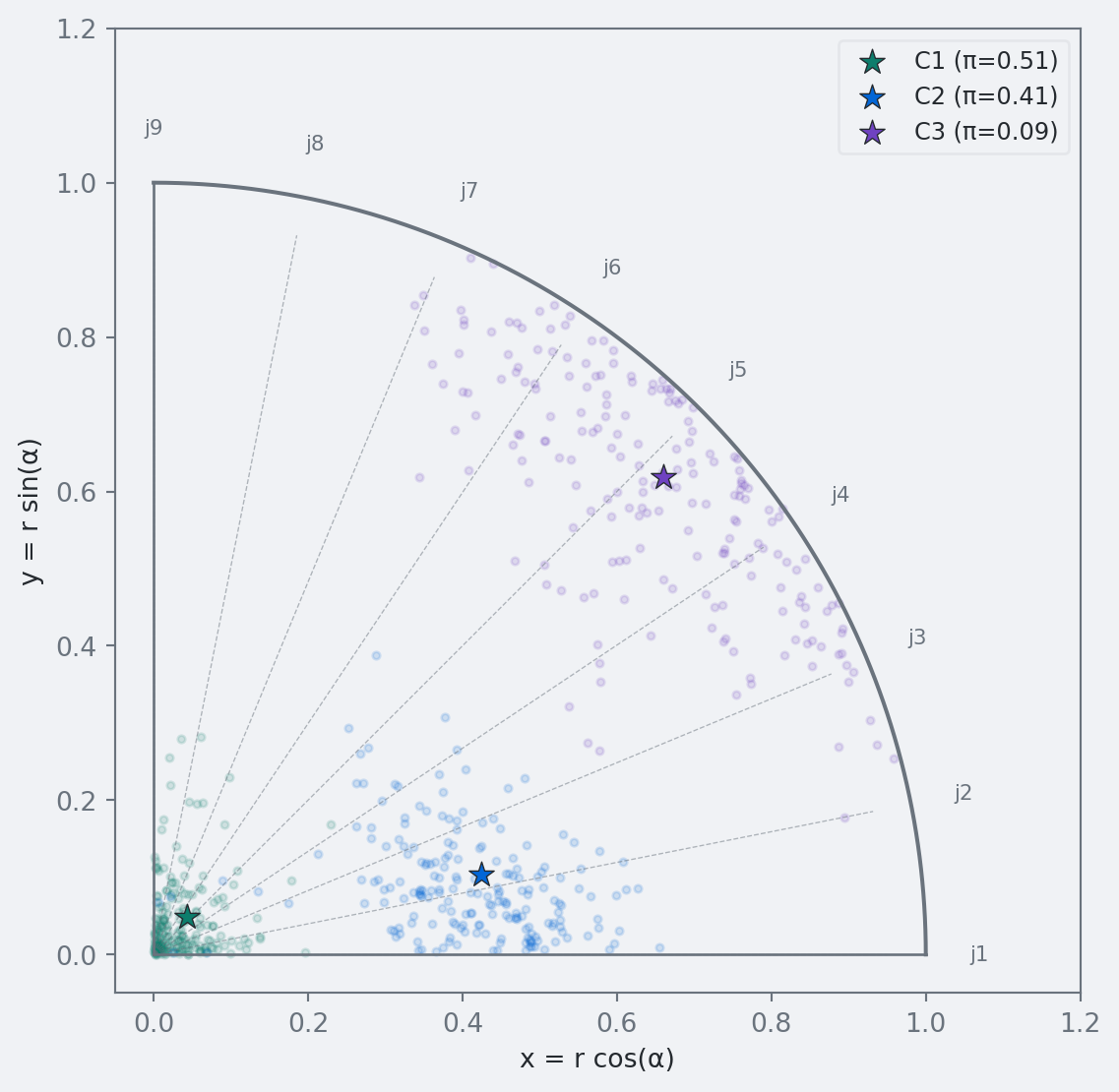
The fitted classes are radially ordered with clear gaps: median radii are about \(r_1=0.05\), \(r_2=0.43\), and \(r_3=0.93\) (see the 90% intervals in the table). Class 3 is near the boundary, while Classes 1 and 2 are well separated low/moderate groups.

5.3 Class Locations on the Disk

Show the code
fig, ax = plt.subplots(figsize=(6, 6))
style_axes(ax, grid=False)

# Unit circle arc
t = np.linspace(0, np.pi/2, 100)
ax.plot(np.cos(t), np.sin(t), color=blog["text_light"], lw=1.5)
ax.plot([0, 1], [0, 0], color=blog["text_light"], lw=1)
ax.plot([0, 0], [0, 1], color=blog["text_light"], lw=1)

# Item directions
phi = np.array([(np.pi/2) * j / (J-1) for j in range(J)])
for j in range(J):
    ax.plot([0, 0.95*np.cos(phi[j])], [0, 0.95*np.sin(phi[j])],
            color=blog["text_light"], lw=0.5, ls='--', alpha=0.5)
    ax.text(1.07*np.cos(phi[j]), 1.07*np.sin(phi[j]), f"j{j+1}",
            ha="center", va="center", fontsize=8, color=blog["text_light"])

# Posterior samples
n_draw = min(200, radii_post.shape[0])
idx = np.random.choice(radii_post.shape[0], n_draw, replace=False)
for k in range(K):
    x_pts = radii_post[idx, k] * np.cos(angles_post[idx, k])
    y_pts = radii_post[idx, k] * np.sin(angles_post[idx, k])
    ax.scatter(x_pts, y_pts, color=colors[k], alpha=0.15, s=8)
    r_m, a_m = radii_post[:, k].mean(), angles_post[:, k].mean()
    ax.scatter(r_m * np.cos(a_m), r_m * np.sin(a_m),
               color=colors[k], s=100, marker="*", edgecolors=blog["text"],
               linewidths=0.5, zorder=5, label=f"C{k+1} (π={pi_mean[k]:.2f})")

ax.set_xlim(-0.05, 1.2)
ax.set_ylim(-0.05, 1.2)
ax.set_aspect("equal")
ax.legend(fontsize=9, loc="upper right")
ax.set_xlabel("x = r cos(α)")
ax.set_ylabel("y = r sin(α)")
plt.tight_layout()
plt.show()
Figure 1: Posterior draws of latent class positions on the restricted Poincaré disk. Stars mark posterior means. Dashed lines show fixed item directions.

5.4 Item Probability Profiles

Show the code
fig, axes = plt.subplots(1, K, figsize=(5*K, 4), sharey=True)
x = np.arange(J)

for k in range(K):
    ax = axes[k]
    style_axes(ax)
    means = theta_post[:, k, :].mean(axis=0)
    q05 = np.percentile(theta_post[:, k, :], 5, axis=0)
    q95 = np.percentile(theta_post[:, k, :], 95, axis=0)
    ax.bar(x, means, 0.6, color=colors[k], alpha=0.5)
    ax.errorbar(x, means, yerr=[means - q05, q95 - means],
                fmt='none', color=colors[k], capsize=3, lw=1.5)
    ax.set_xticks(x)
    ax.set_xticklabels([f"j{j+1}" for j in range(J)], fontsize=8, rotation=45)
    ax.set_ylim(0, 1)
    ax.set_title(f"Class {k+1} (π={pi_mean[k]:.2f})", fontweight="bold")
    if k == 0:
        ax.set_ylabel("P(endorse)")

plt.tight_layout()
plt.show()
Figure 2: Posterior mean item probabilities by class with 90% credible intervals.

5.5 Item Parameters

Show the code
alpha_post = fit.stan_variable('alpha')
lam_post = fit.stan_variable('lam')

fig, (ax1, ax2) = plt.subplots(1, 2, figsize=(10, 4))
style_axes(ax1)
style_axes(ax2)

bp1 = ax1.boxplot([alpha_post[:, j] for j in range(J)], patch_artist=True, widths=0.5)
for patch in bp1['boxes']:
    patch.set_facecolor(blog["blue"])
    patch.set_alpha(0.4)
ax1.set_xticklabels([f"j{j+1}" for j in range(J)], fontsize=8)
ax1.set_ylabel("α (baseline)")
ax1.set_title("Item Baselines", fontweight="bold")
ax1.axhline(0, color=blog["text_light"], ls="--", lw=0.5)

bp2 = ax2.boxplot([lam_post[:, j] for j in range(J)], patch_artist=True, widths=0.5)
for patch in bp2['boxes']:
    patch.set_facecolor(blog["red"])
    patch.set_alpha(0.4)
ax2.set_xticklabels([f"j{j+1}" for j in range(J)], fontsize=8)
ax2.set_ylabel("λ (discrimination)")
ax2.set_title("Item Discriminations", fontweight="bold")

plt.tight_layout()
plt.show()
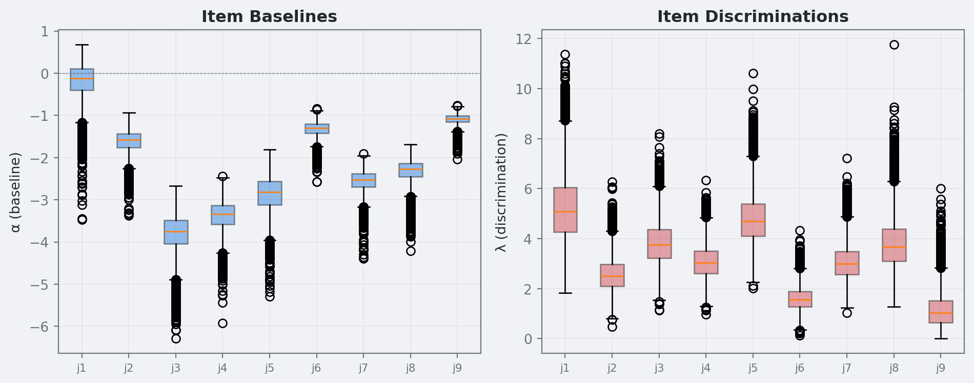
Figure 3: Posterior distributions of item baselines (α) and discriminations (λ).

6. Separation Diagnostics in Hyperbolic Space

The hyperbolic distance between two classes \(a\) and \(b\) on the Poincaré disk is (Nickel and Kiela 2017): \[ d_{\mathbb{H}}(z_a, z_b) = 2\,\operatorname{arctanh}\!\left(\frac{|z_a - z_b|}{|1 - \bar{z}_a z_b|}\right) \] where \(z_k = r_k e^{i\alpha_k}\) is the complex representation of the class position.

6.1 Why This Metric Is Useful

Unlike Euclidean distance, hyperbolic distance grows quickly near the boundary (\(r \to 1\)). That gives three practical diagnostics:

  1. Boundary classes can be strongly distinct. Large \(d_{\mathbb{H}}\) values near the rim indicate genuinely different high-severity profiles.

  2. Central classes are naturally close to all others. A class near \(r\approx0\) tends to have small distance to every class because its profile is close to baseline.

  3. The minimum pairwise distance is an adequacy check. Small \(\min d_{\mathbb{H}}\) suggests redundant classes; larger values support distinct classes for the chosen \(K\).

6.2 Hyperbolic vs Profile Distance

Profile distance (\(\|\boldsymbol{\theta}_a - \boldsymbol{\theta}_b\|_2\)) measures separation in observable item-probability space. Hyperbolic distance measures structural separation in latent space.

The two can disagree. For example, weak discrimination can make geometrically distinct classes look similar in profile space. Using both gives a better separation diagnosis than either metric alone.

Show the code
hyp_post = fit.stan_variable('hyp_dist')
mpd_post = fit.stan_variable('min_profile_dist')
min_hyp_post = fit.stan_variable('min_hyp_dist')

print("Pairwise Hyperbolic Distances (posterior mean):")
hyp_mean = hyp_post.mean(axis=0)
labels = [f"C{k+1}" for k in range(K)]
hyp_df = pd.DataFrame(hyp_mean, index=labels, columns=labels).round(3)
print(hyp_df.to_string())

q = np.percentile(min_hyp_post, [5, 50, 95])
print(f"\nMin hyperbolic distance: {q[1]:.3f}  90% CI = [{q[0]:.3f}, {q[2]:.3f}]")

q2 = np.percentile(mpd_post, [5, 50, 95])
print(f"Min profile distance:   {q2[1]:.3f}  90% CI = [{q2[0]:.3f}, {q2[2]:.3f}]")
Pairwise Hyperbolic Distances (posterior mean):
       C1     C2     C3
C1  0.000  0.868  3.305
C2  0.868  0.000  2.842
C3  3.305  2.842  0.000

Min hyperbolic distance: 0.846  90% CI = [0.537, 1.253]
Min profile distance:   0.491  90% CI = [0.326, 0.605]

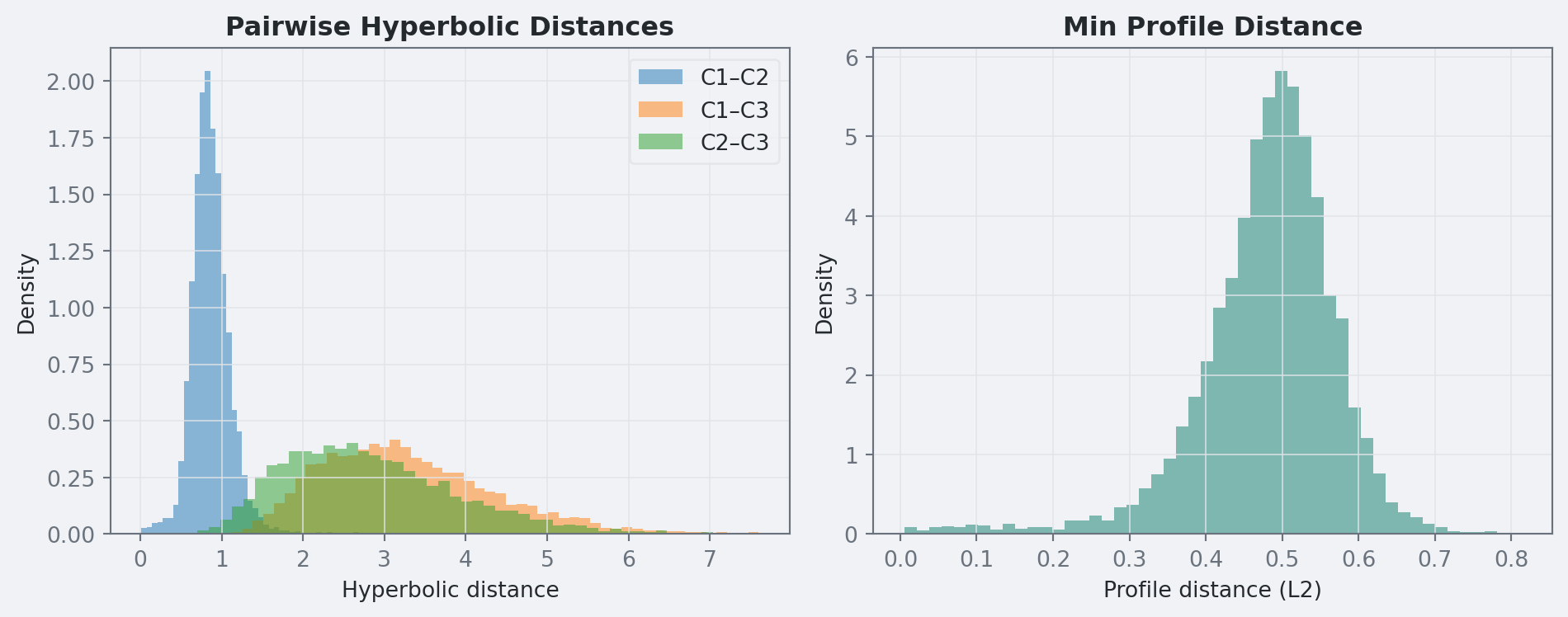
In this run, separation is strong: the minimum pairwise hyperbolic distance has posterior median 0.85 (90% interval [0.54, 1.25]), and the minimum profile distance has median 0.49 (90% interval [0.33, 0.61]).

Show the code
pairs = [(a, b) for a in range(K) for b in range(a+1, K)]

fig, (ax1, ax2) = plt.subplots(1, 2, figsize=(10, 4))
style_axes(ax1)
style_axes(ax2)

for a, b in pairs:
    ax1.hist(hyp_post[:, a, b], bins=50, alpha=0.5, label=f"C{a+1}–C{b+1}", density=True)
ax1.set_xlabel("Hyperbolic distance")
ax1.set_ylabel("Density")
ax1.set_title("Pairwise Hyperbolic Distances", fontweight="bold")
ax1.legend()

ax2.hist(mpd_post, bins=50, alpha=0.5, color=blog["teal"], density=True)
ax2.set_xlabel("Profile distance (L2)")
ax2.set_ylabel("Density")
ax2.set_title("Min Profile Distance", fontweight="bold")

plt.tight_layout()
plt.show()
Figure 4: Posterior distributions of pairwise hyperbolic distances and minimum profile distance.

7. Frequentist Cross-Check with poLCA

As a baseline, I fit the same \(K=3\) model with poLCA in R using many random starts (Linzer and Lewis 2011).

Show the code
if shutil.which("Rscript") is None:
    raise RuntimeError("Rscript is required for poLCA comparison but was not found on PATH.")

r_code = textwrap.dedent(f"""
suppressPackageStartupMessages(library(poLCA))
set.seed(1234)

raw <- read.csv("data/lca1.csv", header=FALSE)
Y <- raw[, -1]
colnames(Y) <- paste0("j", 1:ncol(Y))
for (j in seq_along(Y)) Y[[j]] <- Y[[j]] + 1L

f <- as.formula(paste0("cbind(", paste(colnames(Y), collapse=","), ") ~ 1"))
fit <- poLCA(f, data=Y, nclass={K}, nrep=100, maxiter=5000, tol=1e-10,
             verbose=FALSE, graphs=FALSE)

cat(sprintf("LLIK %.12f\\n", fit$llik))
cat(paste("PI", paste(fit$P, collapse=" "), sep=" "), "\\n")
for (j in seq_len(ncol(Y))) {{
  p <- fit$probs[[paste0("j", j)]][, 2]
  cat(paste0("J", j, " ", paste(p, collapse=" "), "\\n"))
}}
""")

res = subprocess.run(["Rscript", "-e", r_code], check=True, capture_output=True, text=True)
lines = [ln.strip() for ln in res.stdout.splitlines() if ln.strip()]
lines = [ln for ln in lines if ln.startswith("LLIK") or ln.startswith("PI") or ln.startswith("J")]

polca_llik = float(lines[0].split()[1])
freq_pi = np.array([float(x) for x in lines[1].split()[1:]], dtype=float)
freq_theta = np.zeros((K, J))
for ln in lines[2:]:
    parts = ln.split()
    j = int(parts[0][1:]) - 1
    freq_theta[:, j] = np.array([float(x) for x in parts[1:]], dtype=float)

freq_labels = [f"poLCA class {k+1}" for k in range(K)]

# Match classes: Bayes classes are ordered by radius (C1 = smallest r = most baseline)
# We align classes by solving a global assignment problem (Hungarian algorithm)
# on profile distance with a small class-proportion penalty.

# Build comparison table
print("=" * 80)
print("Frequentist (poLCA) vs Bayesian Geometric")
print("=" * 80)

# Global class matching
from scipy.spatial.distance import cdist
from scipy.optimize import linear_sum_assignment

match_weight_pi = 0.25
geo_cost = cdist(theta_mean, freq_theta) + match_weight_pi * np.abs(pi_mean[:, None] - freq_pi[None, :])
geo_idx, freq_idx = linear_sum_assignment(geo_cost)
geo_for_freq = {f: g for g, f in zip(geo_idx, freq_idx)}
matched = [(geo_for_freq[f], f) for f in range(K)]  # ordered by poLCA class index

print(f"\n{'':>25}" + "".join(f"{'j'+str(j+1):>7}" for j in range(J)) + "      π")
print("-" * 80)

for fk in range(K):
    bk = geo_for_freq[fk]
    print(f"  poLCA {freq_labels[fk]:>18}" + "".join(f"{freq_theta[fk,j]:>7.3f}" for j in range(J))
          + f"  {freq_pi[fk]:.3f}")
    print(f"  Geometric C{bk+1:>12}" + "".join(f"{theta_mean[bk,j]:>7.3f}" for j in range(J))
          + f"  {pi_mean[bk]:.3f}")
    print()

print(f"poLCA log-likelihood: {polca_llik:.2f}")
abs_diff = np.abs(theta_mean[[geo_for_freq[f] for f in range(K)], :] - freq_theta)
print(f"Mean absolute item-probability gap (matched classes): {abs_diff.mean():.3f}")
print(f"Max absolute item-probability gap (matched classes):  {abs_diff.max():.3f}")
print("=" * 80)
================================================================================
Frequentist (poLCA) vs Bayesian Geometric
================================================================================

                              j1     j2     j3     j4     j5     j6     j7     j8     j9      π
--------------------------------------------------------------------------------
  poLCA      poLCA class 1  0.909  0.338  0.065  0.066  0.219  0.321  0.113  0.141  0.326  0.557
  Geometric C           2  0.865  0.372  0.105  0.107  0.250  0.305  0.143  0.162  0.273  0.407

  poLCA      poLCA class 2  0.313  0.164  0.036  0.056  0.045  0.183  0.098  0.110  0.188  0.365
  Geometric C           1  0.501  0.184  0.028  0.040  0.072  0.227  0.085  0.108  0.261  0.505

  poLCA      poLCA class 3  0.923  0.549  0.428  0.421  0.775  0.468  0.517  0.619  0.345  0.078
  Geometric C           3  0.949  0.565  0.341  0.332  0.775  0.509  0.467  0.578  0.393  0.088

poLCA log-likelihood: -4229.31
Mean absolute item-probability gap (matched classes): 0.041
Max absolute item-probability gap (matched classes):  0.188
================================================================================
Show the code
fig, axes = plt.subplots(1, K, figsize=(5*K, 4.5), sharey=True)
x = np.arange(J)
w = 0.35

for i, fk in enumerate(range(K)):
    bk = geo_for_freq[fk]
    ax = axes[i]
    style_axes(ax)
    ax.bar(x - w/2, freq_theta[fk], w, color=blog["text_light"], alpha=0.6, label=f"poLCA: {freq_labels[fk]}")
    geo_means = theta_mean[bk]
    q05 = np.percentile(theta_post[:, bk, :], 5, axis=0)
    q95 = np.percentile(theta_post[:, bk, :], 95, axis=0)
    ax.bar(x + w/2, geo_means, w, color=colors[bk], alpha=0.7, label=f"Geometric C{bk+1}")
    ax.errorbar(x + w/2, geo_means, yerr=[geo_means - q05, q95 - geo_means],
                fmt='none', color=blog["text"], capsize=2, lw=0.8)
    ax.set_xticks(x)
    ax.set_xticklabels([f"j{j+1}" for j in range(J)], fontsize=7, rotation=45)
    ax.set_ylim(0, 1)
    ax.legend(fontsize=7, loc="upper right")
    ax.set_title(f"π: poLCA={freq_pi[fk]:.3f} vs NUTS={pi_mean[bk]:.3f}", fontweight="bold")
    if i == 0:
        ax.set_ylabel("P(endorse)")

plt.tight_layout()
plt.show()
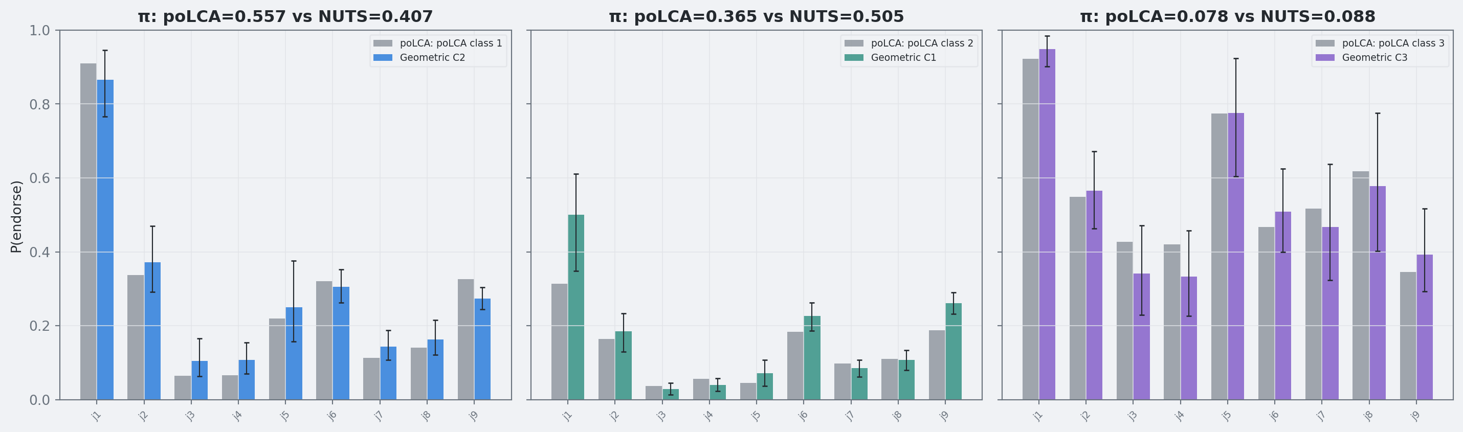
Figure 5: Frequentist poLCA (gray) vs Bayesian geometric (color) item probabilities with 90% credible intervals.

8. What This Run Shows

  • NUTS diagnostics are strong (no divergences, \(\hat{R}\) near 1), so posterior summaries are stable.
  • Class separation is now clear in both latent space and profile space.
  • Matched class proportions are close to poLCA (Bayes about 0.51, 0.41, 0.09 vs poLCA about 0.56, 0.37, 0.08).
  • Remaining mismatch to poLCA is modest (mean absolute item-probability gap about 0.04; maximum about 0.19).

The practical result is that the restricted Poincare specification is now doing what it should: identifiable classes, interpretable geometry, and competitive fit on this dataset.

9. Optional Extension: Geometric Mean with Sparse Departures

The base model constrains all item-class logits to the cosine surface \[ \text{logit}(\theta_{kj}) = \alpha_j + \lambda_j r_k \cos(\alpha_k - \varphi_j). \] This is interpretable, but it can be too rigid in some datasets.

The extension keeps the geometric mean structure and adds sparse deviations with a regularized horseshoe prior (Piironen and Vehtari 2017): \[ \text{logit}(\theta_{kj}) = \mu_{kj} + \delta_{kj}, \qquad \delta_{kj} = z_{kj}\,\tau\,\tilde{\lambda}_{kj} \] where \(\mu_{kj} = \alpha_j + \lambda_j r_k \cos(\alpha_k - \varphi_j)\) is the geometric prediction, \[ z_{kj}\sim\mathcal{N}(0,1),\quad \lambda_{kj}\sim\mathcal{C}^+(0,1),\quad \tau\sim\mathcal{C}^+(0,\tau_0), \] and the regularized local scale is \[ \tilde{\lambda}_{kj} =\sqrt{\frac{c^2\lambda_{kj}^2}{c^2+\tau^2\lambda_{kj}^2}}, \qquad c^2\sim\text{Inv-Gamma}\!\left(\frac{\nu}{2},\frac{\nu}{2}\right). \] This prior shrinks most \(\delta_{kj}\) values toward zero and only allows larger departures where the pure geometry misses local structure.

Class identification still comes from ordered radii. Departures then act as diagnostics for item-class cells that need extra flexibility.

Show the code
model_dep = CmdStanModel(stan_file="lca_poincare_departure.stan")
Show the code
def random_init_departure(K, J, rng):
    init = random_init(K, J, rng)
    init['z_delta'] = (rng.randn(K, J) * 0.1).tolist()
    init['hs_lambda'] = (np.abs(rng.randn(K, J)) * 0.3 + 0.1).tolist()
    init['hs_tau'] = float(np.abs(rng.randn()) * 0.1 + 0.1)
    init['hs_c2_aux'] = float(np.abs(rng.randn()) + 1.0)
    return init

def find_best_optimum_departure(model, stan_data, n_starts=20, seed=42):
    best_opt, best_lp = None, -np.inf
    rng = np.random.RandomState(seed)
    K, J = stan_data['K'], stan_data['J']
    for i in range(n_starts):
        init = random_init_departure(K, J, rng)
        try:
            opt = model.optimize(data=stan_data, inits=init, jacobian=True,
                                 seed=seed + i, show_console=False)
            lp = opt.optimized_params_dict['lp__']
            if lp > best_lp:
                best_lp, best_opt = lp, opt
        except Exception:
            pass
    return best_opt

def opt_to_nuts_init_departure(opt, K, J, jitter=0.02, rng=None):
    if rng is None:
        rng = np.random.RandomState()
    dd = opt.optimized_params_dict
    logit_r = np.sort(np.array([dd[f'logit_r[{k+1}]'] for k in range(K)]) + rng.randn(K) * jitter)
    angle_raw = np.array([dd[f'angle_raw[{k+1}]'] for k in range(K)]) + rng.randn(K) * jitter
    alpha = np.array([dd[f'alpha[{j+1}]'] for j in range(J)]) + rng.randn(J) * jitter
    lam = np.maximum(np.array([dd[f'lam[{j+1}]'] for j in range(J)]) + rng.randn(J) * jitter, 0.01)
    pi_w = np.maximum(np.array([dd[f'pi_w[{k+1}]'] for k in range(K)]) + rng.randn(K) * jitter * 0.1, 0.01)
    pi_w /= pi_w.sum()
    z_delta = np.array([[dd[f'z_delta[{k+1},{j+1}]'] for j in range(J)] for k in range(K)])
    hs_lambda = np.array([[dd[f'hs_lambda[{k+1},{j+1}]'] for j in range(J)] for k in range(K)])
    hs_tau = max(dd['hs_tau'] + rng.randn() * jitter * 0.2, 1e-3)
    hs_c2_aux = max(dd['hs_c2_aux'] + rng.randn() * jitter * 0.5, 1e-3)
    return dict(logit_r=logit_r.tolist(), angle_raw=angle_raw.tolist(),
                alpha=alpha.tolist(), lam=lam.tolist(), pi_w=pi_w.tolist(),
                z_delta=(z_delta + rng.randn(K, J) * jitter).tolist(),
                hs_lambda=np.maximum(hs_lambda + rng.randn(K, J) * jitter, 0.01).tolist(),
                hs_tau=float(hs_tau), hs_c2_aux=float(hs_c2_aux))
Show the code
best_opt_dep = find_best_optimum_departure(model_dep, stan_data, n_starts=20, seed=42)
d_dep = best_opt_dep.optimized_params_dict
print(f"Geometric model MAP lp__:  {d['lp__']:.2f}")
print(f"Departure model MAP lp__:  {d_dep['lp__']:.2f}")
print(f"Difference:                {d_dep['lp__'] - d['lp__']:.2f}")
sd_total = sum(abs(d_dep[f'sigma_delta[{k+1},{j+1}]']) for k in range(K) for j in range(J))
print(f"\nMAP total |δ|:            {sd_total:.4f}")
print(f"MAP horseshoe τ:           {d_dep['hs_tau']:.4f}")
print(f"MAP horseshoe slab aux:    {d_dep['hs_c2_aux']:.4f}")
print(f"\nMAP departures δ[k,j] (regularized horseshoe):")
print(f"  {'':>30s}" + "".join(f"{'j'+str(j+1):>8}" for j in range(J)))
for k in range(K):
    vals = [d_dep[f'sigma_delta[{k+1},{j+1}]'] for j in range(J)]
    print(f"  {'C'+str(k+1):>30s}" + "".join(f"{v:>8.4f}" for v in vals))

chains_dep = 4
inits_dep = [opt_to_nuts_init_departure(best_opt_dep, K, J, jitter=0.02 + 0.01*c,
                                         rng=np.random.RandomState(42 + c + 300))
             for c in range(chains_dep)]

fit_dep = model_dep.sample(
    data=stan_data, chains=chains_dep,
    iter_warmup=3000, iter_sampling=2000,
    seed=42, inits=inits_dep,
    adapt_delta=0.98, max_treedepth=12,
    show_progress=False,
)
10:20:36 - cmdstanpy - INFO - Chain [1] start processing
10:20:36 - cmdstanpy - INFO - Chain [1] done processing
10:20:36 - cmdstanpy - INFO - Chain [1] start processing
10:20:36 - cmdstanpy - INFO - Chain [1] done processing
10:20:36 - cmdstanpy - INFO - Chain [1] start processing
10:20:36 - cmdstanpy - INFO - Chain [1] done processing
10:20:36 - cmdstanpy - INFO - Chain [1] start processing
10:20:36 - cmdstanpy - INFO - Chain [1] done processing
10:20:36 - cmdstanpy - INFO - Chain [1] start processing
10:20:36 - cmdstanpy - INFO - Chain [1] done processing
10:20:36 - cmdstanpy - INFO - Chain [1] start processing
10:20:36 - cmdstanpy - INFO - Chain [1] done processing
10:20:36 - cmdstanpy - INFO - Chain [1] start processing
10:20:36 - cmdstanpy - INFO - Chain [1] done processing
10:20:36 - cmdstanpy - INFO - Chain [1] start processing
10:20:36 - cmdstanpy - INFO - Chain [1] done processing
10:20:36 - cmdstanpy - INFO - Chain [1] start processing
10:20:36 - cmdstanpy - INFO - Chain [1] done processing
10:20:36 - cmdstanpy - INFO - Chain [1] start processing
10:20:36 - cmdstanpy - INFO - Chain [1] done processing
10:20:36 - cmdstanpy - INFO - Chain [1] start processing
10:20:36 - cmdstanpy - INFO - Chain [1] done processing
10:20:36 - cmdstanpy - INFO - Chain [1] start processing
10:20:36 - cmdstanpy - INFO - Chain [1] done processing
10:20:36 - cmdstanpy - INFO - Chain [1] start processing
10:20:36 - cmdstanpy - INFO - Chain [1] done processing
10:20:36 - cmdstanpy - INFO - Chain [1] start processing
10:20:36 - cmdstanpy - INFO - Chain [1] done processing
10:20:36 - cmdstanpy - INFO - Chain [1] start processing
10:20:36 - cmdstanpy - INFO - Chain [1] done processing
10:20:36 - cmdstanpy - INFO - Chain [1] start processing
10:20:36 - cmdstanpy - INFO - Chain [1] done processing
10:20:36 - cmdstanpy - INFO - Chain [1] start processing
10:20:36 - cmdstanpy - INFO - Chain [1] done processing
10:20:36 - cmdstanpy - INFO - Chain [1] start processing
10:20:36 - cmdstanpy - INFO - Chain [1] done processing
10:20:36 - cmdstanpy - INFO - Chain [1] start processing
10:20:36 - cmdstanpy - INFO - Chain [1] done processing
10:20:36 - cmdstanpy - INFO - Chain [1] start processing
10:20:36 - cmdstanpy - INFO - Chain [1] done processing
10:20:36 - cmdstanpy - INFO - CmdStan start processing
10:20:36 - cmdstanpy - INFO - Chain [1] start processing
10:20:36 - cmdstanpy - INFO - Chain [2] start processing
10:20:36 - cmdstanpy - INFO - Chain [3] start processing
10:20:36 - cmdstanpy - INFO - Chain [4] start processing
Geometric model MAP lp__:  -4246.63
Departure model MAP lp__:  -4274.26
Difference:                -27.63

MAP total |δ|:            1.3205
MAP horseshoe τ:           0.2048
MAP horseshoe slab aux:    1.0727

MAP departures δ[k,j] (regularized horseshoe):
                                      j1      j2      j3      j4      j5      j6      j7      j8      j9
                              C1 -0.0441 -0.0028  0.0204  0.0558 -0.0334 -0.0588  0.0366  0.0136 -0.1448
                              C2  0.0673  0.0049 -0.0581 -0.1044  0.0332  0.1001 -0.0513 -0.0229  0.2180
                              C3 -0.0232 -0.0021  0.0376  0.0486  0.0002 -0.0413  0.0147  0.0092 -0.0731
10:20:57 - cmdstanpy - INFO - Chain [2] done processing
10:20:58 - cmdstanpy - INFO - Chain [3] done processing
10:21:03 - cmdstanpy - INFO - Chain [1] done processing
10:21:09 - cmdstanpy - INFO - Chain [4] done processing
Show the code
diag_dep = fit_dep.diagnose()
for line in diag_dep.split('\n'):
    if line.strip():
        print(line)
Checking sampler transitions treedepth.
Treedepth satisfactory for all transitions.
Checking sampler transitions for divergences.
No divergent transitions found.
Checking E-BFMI - sampler transitions HMC potential energy.
E-BFMI satisfactory.
Rank-normalized split effective sample size satisfactory for all parameters.
Rank-normalized split R-hat values satisfactory for all parameters.
Processing complete, no problems detected.

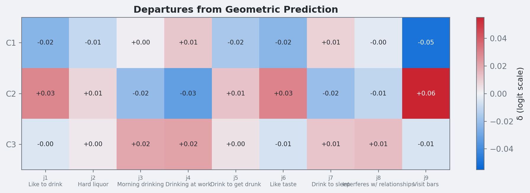
Horseshoe Sparsity Diagnostics

The regularized horseshoe does not hard-threshold coefficients, but shrinks most departures toward zero and allows a few larger effects. Though this extension isn’t helpful in this dataset, it might be useful for more complex data scenarios.

Show the code
delta_post = fit_dep.stan_variable('sigma_delta')  # K×J departure (= delta)
l1_norm = np.abs(delta_post).sum(axis=(1, 2))  # per-draw L1 norm
q = np.percentile(l1_norm, [5, 50, 95])
tau_post = fit_dep.stan_variable('hs_tau')
q_tau = np.percentile(tau_post, [5, 50, 95])
print(f"Posterior horseshoe τ: {q_tau[1]:.4f} [{q_tau[0]:.4f}, {q_tau[2]:.4f}]")
print(f"Posterior total |δ|:   {q[1]:.4f} [{q[0]:.4f}, {q[2]:.4f}]")
n_material = (np.abs(delta_post) > 0.05).sum(axis=(1, 2))
q_mat = np.percentile(n_material, [5, 50, 95])
print(f"Entries with |δ| > 0.05 (of {K*J}): {q_mat[1]:.0f} [{q_mat[0]:.0f}, {q_mat[2]:.0f}]")
Posterior horseshoe τ: 0.0912 [0.0097, 0.2326]
Posterior total |δ|:   1.2429 [0.1282, 3.3400]
Entries with |δ| > 0.05 (of 27): 9 [0, 20]

Departure Heatmap

Show the code
delta_post = fit_dep.stan_variable('delta')  # = sigma_delta
delta_mean = delta_post.mean(axis=0)

fig, ax = plt.subplots(figsize=(10, 3.5))
style_axes(ax, grid=False)
vmax = np.abs(delta_mean).max()
blog_div = LinearSegmentedColormap.from_list(
    "blog_div",
    [blog["blue"], blog["background"], blog["red"]],
)
im = ax.imshow(delta_mean, cmap=blog_div, vmin=-vmax, vmax=vmax, aspect='auto')
ax.set_xticks(range(J))
ax.set_xticklabels([f"j{j+1}\n{item_labels[j]}" for j in range(J)], fontsize=7)
ax.set_yticks(range(K))
ax.set_yticklabels([f"C{k+1}" for k in range(K)])
for k in range(K):
    for j in range(J):
        ax.text(j, k, f"{delta_mean[k,j]:+.2f}", ha='center', va='center', fontsize=8,
                color='white' if abs(delta_mean[k,j]) > vmax*0.6 else blog["text"])
cbar = plt.colorbar(im, ax=ax, label="δ (logit scale)")
cbar.outline.set_edgecolor(blog["text_light"])
cbar.ax.yaxis.label.set_color(blog["text"])
cbar.ax.tick_params(color=blog["text_light"], labelcolor=blog["text_light"])
cbar.ax.set_facecolor(blog["background"])
ax.set_title("Departures from Geometric Prediction", fontweight="bold")
plt.tight_layout()
plt.show()
Figure 6: Posterior mean departures δ[k,j] = logit(θ) − geometric prediction. Red = item-class pair endorses more than geometry predicts; blue = less.

Model Comparison via LOO

Show the code
import importlib.util
import warnings
warnings.filterwarnings("ignore")

if importlib.util.find_spec("arviz") is None:
    print("Skipping LOO comparison: 'arviz' is not installed in the active Python environment.")
else:
    import arviz as az

    def make_loo_idata(fit_obj, cnt):
        ll_pattern = fit_obj.stan_variable('log_lik')
        ll_obs = np.repeat(ll_pattern, cnt, axis=1)
        n_chains = fit_obj.chains
        n_draws = fit_obj.num_draws_sampling
        ll_3d = ll_obs.reshape(n_chains, n_draws, -1)
        return az.from_dict(
            log_likelihood={"y": ll_3d},
            posterior={"mu": np.zeros((n_chains, n_draws))}
        )

    idata_geo = make_loo_idata(fit, cnt)
    idata_dep = make_loo_idata(fit_dep, cnt)

    loo_geo = az.loo(idata_geo)
    loo_dep = az.loo(idata_dep)

    print(f"Geometric model ELPD (LOO): {loo_geo.elpd_loo:.1f} ± {loo_geo.se:.1f}")
    print(f"Departure model ELPD (LOO): {loo_dep.elpd_loo:.1f} ± {loo_dep.se:.1f}")
    print(f"Difference:                 {loo_dep.elpd_loo - loo_geo.elpd_loo:.1f}")
Geometric model ELPD (LOO): -4261.6 ± 56.6
Departure model ELPD (LOO): -4260.4 ± 56.6
Difference:                 1.2

Three-Way Comparison: Class Proportions

Show the code
theta_dep_post = fit_dep.stan_variable('theta')
theta_dep_mean = theta_dep_post.mean(axis=0)
pi_dep_post = fit_dep.stan_variable('pi_w')
pi_dep_mean = pi_dep_post.mean(axis=0)

# Match departure classes directly to poLCA classes using the same cost function
dep_cost = cdist(theta_dep_mean, freq_theta) + match_weight_pi * np.abs(pi_dep_mean[:, None] - freq_pi[None, :])
dep_idx, dep_freq_idx = linear_sum_assignment(dep_cost)
dep_for_freq = {f: d for d, f in zip(dep_idx, dep_freq_idx)}

class_rows = []
for fk in range(K):
    bk = geo_for_freq[fk]
    depk = dep_for_freq[fk]

    pi_geo_q = np.percentile(pi_post[:, bk], [5, 50, 95])
    pi_dep_q = np.percentile(pi_dep_post[:, depk], [5, 50, 95])

    class_rows.append({
        "Class": f"{freq_labels[fk]}",
        "poLCA π": f"{freq_pi[fk]:.3f}",
        "Geometric class": f"C{bk+1}",
        "Geometric π": f"{pi_geo_q[1]:.3f} [{pi_geo_q[0]:.3f}, {pi_geo_q[2]:.3f}]",
        "Departure class": f"C{depk+1}",
        "Departure π": f"{pi_dep_q[1]:.3f} [{pi_dep_q[0]:.3f}, {pi_dep_q[2]:.3f}]",
    })

pd.DataFrame(class_rows).set_index("Class")
poLCA π Geometric class Geometric π Departure class Departure π
Class
poLCA class 1 0.557 C2 0.403 [0.206, 0.617] C2 0.426 [0.225, 0.626]
poLCA class 2 0.365 C1 0.510 [0.281, 0.710] C1 0.488 [0.277, 0.690]
poLCA class 3 0.078 C3 0.084 [0.044, 0.151] C3 0.082 [0.046, 0.144]

Three-Way Comparison: Item Probabilities

Show the code
for fk in range(K):
    bk = geo_for_freq[fk]
    depk = dep_for_freq[fk]
    print(f"\n{'='*95}")
    print(f"  {freq_labels[fk]}  (Geo=C{bk+1}, Dep=C{depk+1})")
    print(f"{'='*95}")
    print(f"  {'':>12}" + "".join(f"{'j'+str(j+1):>10}" for j in range(J)))
    print(f"  {'-'*93}")

    # poLCA
    print(f"  {'poLCA':>12}" + "".join(f"{freq_theta[fk,j]:>10.3f}" for j in range(J)))

    # Geometric with CI
    geo_q05 = np.percentile(theta_post[:, bk, :], 5, axis=0)
    geo_q95 = np.percentile(theta_post[:, bk, :], 95, axis=0)
    print(f"  {'Geometric':>12}" + "".join(f"{theta_mean[bk,j]:>10.3f}" for j in range(J)))
    print(f"  {'90% CI':>12}" + "".join(
        f"{'['+f'{geo_q05[j]:.2f}'+','+f'{geo_q95[j]:.2f}'+']':>10}" for j in range(J)))

    # Departure with CI
    dep_q05 = np.percentile(theta_dep_post[:, depk, :], 5, axis=0)
    dep_q95 = np.percentile(theta_dep_post[:, depk, :], 95, axis=0)
    print(f"  {'Departure':>12}" + "".join(f"{theta_dep_mean[depk,j]:>10.3f}" for j in range(J)))
    print(f"  {'90% CI':>12}" + "".join(
        f"{'['+f'{dep_q05[j]:.2f}'+','+f'{dep_q95[j]:.2f}'+']':>10}" for j in range(J)))

===============================================================================================
  poLCA class 1  (Geo=C2, Dep=C2)
===============================================================================================
                      j1        j2        j3        j4        j5        j6        j7        j8        j9
  ---------------------------------------------------------------------------------------------
         poLCA     0.909     0.338     0.065     0.066     0.219     0.321     0.113     0.141     0.326
     Geometric     0.865     0.372     0.105     0.107     0.250     0.305     0.143     0.162     0.273
        90% CI[0.77,0.95][0.29,0.47][0.06,0.17][0.07,0.15][0.16,0.38][0.26,0.35][0.11,0.19][0.12,0.22][0.24,0.30]
     Departure     0.866     0.368     0.101     0.103     0.245     0.308     0.140     0.159     0.283
        90% CI[0.78,0.94][0.29,0.46][0.06,0.15][0.07,0.15][0.16,0.36][0.26,0.36][0.11,0.18][0.12,0.21][0.25,0.33]

===============================================================================================
  poLCA class 2  (Geo=C1, Dep=C1)
===============================================================================================
                      j1        j2        j3        j4        j5        j6        j7        j8        j9
  ---------------------------------------------------------------------------------------------
         poLCA     0.313     0.164     0.036     0.056     0.045     0.183     0.098     0.110     0.188
     Geometric     0.501     0.184     0.028     0.040     0.072     0.227     0.085     0.108     0.261
        90% CI[0.35,0.61][0.13,0.23][0.01,0.05][0.02,0.06][0.04,0.11][0.19,0.26][0.06,0.11][0.08,0.13][0.23,0.29]
     Departure     0.485     0.180     0.028     0.040     0.069     0.221     0.086     0.108     0.252
        90% CI[0.33,0.60][0.13,0.23][0.01,0.04][0.02,0.06][0.04,0.10][0.18,0.26][0.06,0.11][0.08,0.13][0.21,0.29]

===============================================================================================
  poLCA class 3  (Geo=C3, Dep=C3)
===============================================================================================
                      j1        j2        j3        j4        j5        j6        j7        j8        j9
  ---------------------------------------------------------------------------------------------
         poLCA     0.923     0.549     0.428     0.421     0.775     0.468     0.517     0.619     0.345
     Geometric     0.949     0.565     0.341     0.332     0.775     0.509     0.467     0.578     0.393
        90% CI[0.90,0.98][0.46,0.67][0.23,0.47][0.23,0.46][0.60,0.92][0.40,0.62][0.32,0.64][0.40,0.78][0.29,0.52]
     Departure     0.948     0.563     0.345     0.338     0.777     0.505     0.472     0.582     0.389
        90% CI[0.90,0.98][0.46,0.67][0.23,0.48][0.23,0.46][0.62,0.92][0.39,0.62][0.34,0.64][0.41,0.77][0.29,0.51]
Show the code
fig, axes = plt.subplots(1, K, figsize=(5*K, 4.5), sharey=True)
x = np.arange(J)
w = 0.27

for i, fk in enumerate(range(K)):
    bk = geo_for_freq[fk]
    depk = dep_for_freq[fk]
    ax = axes[i]
    style_axes(ax)
    ax.bar(x - w, freq_theta[fk], w, color=blog["text_light"], alpha=0.6, label=f"poLCA: {freq_labels[fk]}")

    geo_means = theta_mean[bk]
    geo_q05 = np.percentile(theta_post[:, bk, :], 5, axis=0)
    geo_q95 = np.percentile(theta_post[:, bk, :], 95, axis=0)
    ax.bar(x, geo_means, w, color=colors[bk], alpha=0.35, label=f"Geometric C{bk+1}")
    ax.errorbar(x, geo_means, yerr=[geo_means - geo_q05, geo_q95 - geo_means],
                fmt='none', color=blog["text"], capsize=2, lw=0.8)

    dep_means = theta_dep_mean[depk]
    dep_q05 = np.percentile(theta_dep_post[:, depk, :], 5, axis=0)
    dep_q95 = np.percentile(theta_dep_post[:, depk, :], 95, axis=0)
    ax.bar(x + w, dep_means, w, color=colors[bk], alpha=0.8, label=f"Departure C{depk+1}")
    ax.errorbar(x + w, dep_means, yerr=[dep_means - dep_q05, dep_q95 - dep_means],
                fmt='none', color=blog["text"], capsize=2, lw=0.8)

    ax.set_xticks(x)
    ax.set_xticklabels([f"j{j+1}" for j in range(J)], fontsize=7, rotation=45)
    ax.set_ylim(0, 1)
    ax.legend(fontsize=6, loc="upper right")
    ax.set_title(f"π: poLCA={freq_pi[fk]:.3f}, Geo={pi_mean[bk]:.3f}, Dep={pi_dep_mean[depk]:.3f}",
                 fontweight="bold", fontsize=9)
    if i == 0:
        ax.set_ylabel("P(endorse)")

plt.tight_layout()
plt.show()
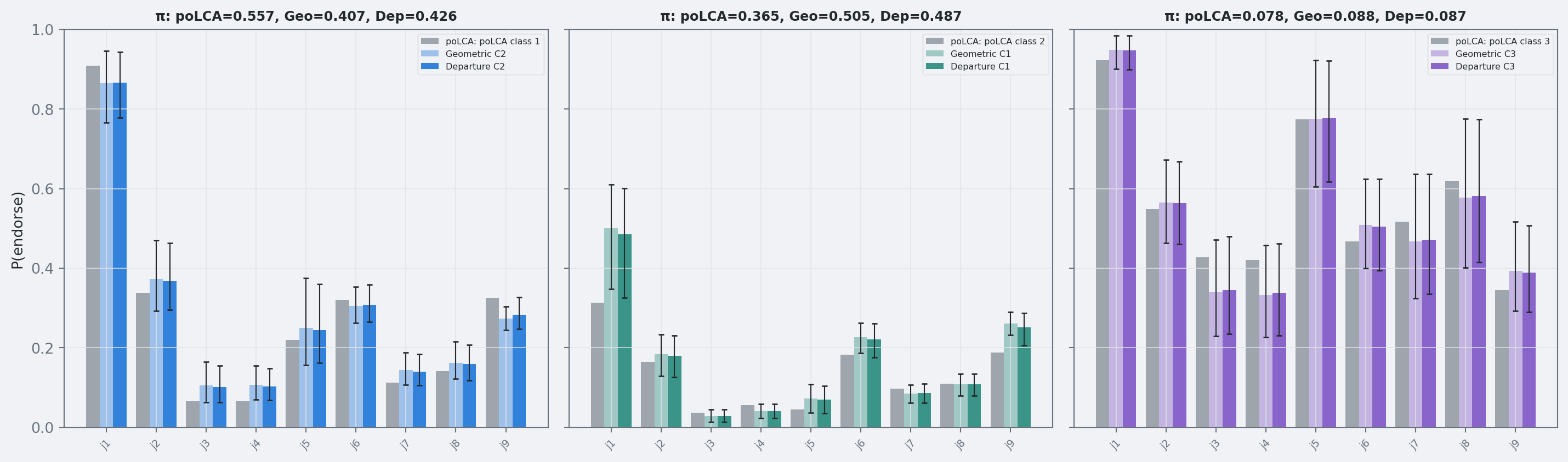
Figure 7: Three-way comparison: poLCA (gray), geometric (light), and departure model (saturated) item probabilities with 90% credible intervals.

Appendix: Stan Code

lca_poincare.stan
// lca_poincare.stan
// LCA with Restricted Cosine Poincaré Disk + BLAS matmul likelihood
// =================================================================
//
// theta[k,j] = inv_logit(alpha[j] + lam[j] * r[k] * cos(angle[k] - phi[j]))
//
// Items spread evenly at phi[j] = (π/2)(j-1)/(J-1) in [0, π/2].
// Classes identified by ordered radii.
//
// Likelihood uses BLAS matmul: S = Y * η' avoids inner loop over items.

data {
  int<lower=1> P;                              // unique response patterns
  int<lower=2> K;                              // latent classes
  int<lower=2> J;                              // items (≥2 for phi spacing)
  array[P, J] int<lower=0, upper=1> pattern;  // unique binary patterns
  array[P] int<lower=1> count;                 // count per pattern
}

transformed data {
  int N = sum(count);
  vector[J] phi;
  for (j in 1:J)
    phi[j] = (pi() / 2) * (j - 1.0) / (J - 1.0);

  // Real matrix version of pattern for BLAS matmul
  matrix[P, J] Y;
  for (p in 1:P)
    for (j in 1:J)
      Y[p, j] = pattern[p, j];

  row_vector[J] rv = rep_row_vector(1.0, J);
}

parameters {
  ordered[K] logit_r;           // ordered logit-radii → identifiability
  vector[K] angle_raw;          // mapped to (0, pi/2) via scaled logistic
  vector[J] alpha;              // item baselines
  vector<lower=0>[J] lam;      // item discriminations
  simplex[K] pi_w;             // mixing weights
}

transformed parameters {
  vector<lower=0, upper=1>[K] radii;
  vector<lower=0>[K] angles;
  matrix[K, J] logit_theta;    // η[k,j] = alpha[j] + lam[j] * r[k] * cos(a[k] - phi[j])
  // matrix[K, J] theta;

  for (k in 1:K) {
    radii[k] = inv_logit(logit_r[k]);
    angles[k] = (pi() / 2) * inv_logit(angle_raw[k]);
  }

  for (k in 1:K)
    for (j in 1:J) {
      logit_theta[k, j] = alpha[j] + lam[j] * radii[k] * cos(angles[k] - phi[j]);
     // theta[k, j] = inv_logit(logit_theta[k, j]);
    }
}

model {
  // Priors
  logit_r ~ normal(0, 2);
  angle_raw ~ normal(0, 2);
  alpha ~ normal(0, 3);
  lam ~ normal(0, 3);           // half-normal via <lower=0>
  pi_w ~ dirichlet(rep_vector(2.0, K));

  // --- fast marginalized mixture likelihood ---
  {
    // For each class k:
    //   Σ_j log p(y_j | η_j,k)
    // = (y^T η_:,k) - Σ_j log(1+exp η_j,k)
    row_vector[K] sum_log1p = rv * log1p_exp(logit_theta'); // length K
    vector[K] c = -sum_log1p';
    vector[K] log_nu = log(pi_w);

    // S[p,k] = Σ_j Y[p,j] * η[k,j]  (BLAS matmul)
    matrix[P, K] S = Y * logit_theta';

    for (p in 1:P)
      target += count[p] * log_sum_exp(log_nu + (S[p]' + c));
  }

  // --- sufficient-statistics likelihood (loop version) ---
  // {
  //   matrix[K, J] lt = log(theta);
  //   matrix[K, J] lt1m = log1m(theta);
  //
  //   for (p in 1:P) {
  //     vector[K] lps;
  //     for (k in 1:K) {
  //       lps[k] = log(pi_w[k]);
  //       for (j in 1:J)
  //         lps[k] += pattern[p, j] == 1 ? lt[k, j] : lt1m[k, j];
  //     }
  //     target += count[p] * log_sum_exp(lps);
  //   }
  // }
}

generated quantities {
  vector[P] log_lik;
  matrix[K, J] theta_free;     // relaxed (unconstrained) item probs
  real min_profile_dist;
  matrix[K, K] hyp_dist;
  real min_hyp_dist;

  // Per-pattern log-lik (BLAS version) + responsibilities for theta_free
  {
    row_vector[K] sum_log1p = rv * log1p_exp(logit_theta');
    vector[K] c = -sum_log1p';
    vector[K] log_nu = log(pi_w);
    matrix[P, K] S = Y * logit_theta';

    // log-lik
    for (p in 1:P)
      log_lik[p] = log_sum_exp(log_nu + (S[p]' + c));

    // Relaxed theta via iterated EM (seeded from geometric model)
    // Initial E-step uses geometric logit_theta; then iterate M→E→M...
    {
      // Seed theta_free from geometric model
      matrix[K, J] eta = logit_theta;

      for (em_iter in 1:200) {
        // E-step: responsibilities from current eta
        matrix[P, K] W;
        {
          row_vector[K] slp = rv * log1p_exp(eta');
          vector[K] cc = -slp';
          matrix[P, K] SS = Y * eta';

          for (p in 1:P) {
            vector[K] lp = log_nu + SS[p]' + cc;
            real lse = log_sum_exp(lp);
            for (k in 1:K)
              W[p, k] = count[p] * exp(lp[k] - lse);
          }
        }

        // M-step: theta_free = weighted sample means
        matrix[K, J] numer = W' * Y;
        for (k in 1:K) {
          real denom = sum(W[, k]);
          for (j in 1:J) {
            theta_free[k, j] = numer[k, j] / denom;
            // Update eta for next E-step (logit scale, clamp to avoid ±inf)
            eta[k, j] = log(fmax(theta_free[k, j], 1e-8))
                       - log(fmax(1 - theta_free[k, j], 1e-8));
          }
        }
      }
    }
  }

  // Min pairwise profile distance
  min_profile_dist = positive_infinity();
  for (a in 1:K)
    for (b in (a + 1):K) {
      real d = 0;
      for (j in 1:J)
        d += square(inv_logit(logit_theta[a, j]) - inv_logit(logit_theta[b, j]));
      if (sqrt(d) < min_profile_dist)
        min_profile_dist = sqrt(d);
    }

  // Pairwise hyperbolic distances on Poincaré disk
  for (a in 1:K) {
    hyp_dist[a, a] = 0;
    for (b in (a + 1):K) {
      real xa = radii[a] * cos(angles[a]);
      real ya = radii[a] * sin(angles[a]);
      real xb = radii[b] * cos(angles[b]);
      real yb = radii[b] * sin(angles[b]);
      real num = sqrt(square(xa - xb) + square(ya - yb));
      real re = 1 - (xa * xb + ya * yb);
      real im = -(xa * yb - ya * xb);
      real den = sqrt(square(re) + square(im));
      hyp_dist[a, b] = 2 * atanh(fmin(num / den, 0.999));
      hyp_dist[b, a] = hyp_dist[a, b];
    }
  }

  min_hyp_dist = positive_infinity();
  for (a in 1:K)
    for (b in (a + 1):K)
      if (hyp_dist[a, b] < min_hyp_dist)
        min_hyp_dist = hyp_dist[a, b];
}

References

Carpenter, Bob, Andrew Gelman, Matthew D. Hoffman, Daniel Lee, Ben Goodrich, Michael Betancourt, Marcus Brubaker, Jiqiang Guo, Peter Li, and Allen Riddell. 2017. “Stan: A Probabilistic Programming Language.” Journal of Statistical Software 76 (1): 1–32. https://doi.org/10.18637/jss.v076.i01.
Jasra, Ajay, Christopher C. Holmes, and David A. Stephens. 2005. “Markov Chain Monte Carlo Methods and the Label Switching Problem in Bayesian Mixture Modeling.” Statistical Science 20 (1): 50–67. https://doi.org/10.1214/088342305000000016.
Linzer, Drew A., and Jeffrey B. Lewis. 2011. “poLCA: An r Package for Polytomous Variable Latent Class Analysis.” Journal of Statistical Software 42 (10): 1–29. https://doi.org/10.18637/jss.v042.i10.
Nickel, Maximilian, and Douwe Kiela. 2017. “Poincare Embeddings for Learning Hierarchical Representations.” In Advances in Neural Information Processing Systems 30.
Piironen, Juho, and Aki Vehtari. 2017. “Sparsity Information and Regularization in the Horseshoe and Other Shrinkage Priors.” Electronic Journal of Statistics 11 (2): 5018–51. https://doi.org/10.1214/17-EJS1337SI.
Stephens, Matthew. 2000. “Dealing with Label Switching in Mixture Models.” Journal of the Royal Statistical Society Series B 62 (4): 795–809. https://doi.org/10.1111/1467-9868.00265.
UCLA Statistical Consulting Group. 2026. “Latent Class Analysis.” https://stats.oarc.ucla.edu/sas/dae/latent-class-analysis/.