The Hyper-Tanh Peel: A Novel Parameterization for Unit Vectors
stan
parameterizations
Author
Sean Pinkney
Published
January 15, 2026
1. Introduction
Parameterizing unit vectors (points on a hypersphere \(S^{K-1}\)) in Bayesian models presents unique challenges.
Hyperspherical coordinates (angles) involve boundaries (\(0, \pi\)) that hinder Hamiltonian Monte Carlo (HMC) sampling.
Muller (1959)’s method (normalizing standard Gaussians, how Stan parameterizes unit_vector) is isotropic but over-parameterized (\(K\) parameters for \(K-1\) dimensions) and suffers from a gradient singularity at the origin.
I’m calling this the hyper-tanh peel bijective parameterization. It is a mapping \(\mathbb{R}^{K-1} \to S^{K-1}\). It uses “Logistic Geometry” to create a smooth, unconstrained manifold that is numerically stable and avoids the singularities of traditional methods.
2. Mathematical Formulation
The Transformation
The method “peels” dimensions one by one using the hyperbolic tangent function (\(\tanh\)), which maps \((-\infty, \infty) \to (-1, 1)\), and closes the remaining 2D subspace with a stereographic projection.
This implies that: 1. The peeling parameters follow a sech distribution: \(p(x_i) \propto \text{sech}^{K-i}(x_i)\). 2. The core parameter follows a cauchy distribution: \(p(x_{K-1}) \propto (1+x_{K-1}^2)^{-1}\).
3. Logistic Geometry & Gradient Stability
A problem with Muller (1959)’s method when used with HMC is the singularity at the origin. In Muller’s parameterization, \(\mathbf{y} = \mathbf{z} / \|\mathbf{z}\|\). As \(\mathbf{z} \to 0\), the gradient \(\nabla_\mathbf{z} \mathbf{y}\) explodes to infinity. This creates a “funnel” that traps HMC samplers.
Advantages of this parameterization: The Hyper-Tanh Peel maps the origin of the parameter space \(\mathbf{x}=\mathbf{0}\) to the “North Pole” of the sphere \(\mathbf{y}=(1, 0, \dots, 0)\).
The derivative of the mapping is governed by \(\frac{d}{dx} \tanh(x) = \text{sech}^2(x)\). * At \(x=0\), \(\text{sech}^2(0) = 1\). * The gradient is linear and bounded. There is no singularity.
4. Visual Verification
This demonstrates two key properties using R: 1. Uniformity: With Jacobian correction, Hyper-Tanh matches Muller (1959)’s isotropy. 2. Stability: Hyper-Tanh has bounded gradients where Muller explodes.
Code
library(ggplot2)library(patchwork)library(dplyr)library(tidyr)# Load blog themesource("../../R/theme_blog.R")# --- Define Methods ---# 1. Muller's Method (Standard)generate_muller <-function(N, K=3) { z <-matrix(rnorm(N * K), ncol=K) y <- z /sqrt(rowSums(z^2))return(data.frame(y, Method="Muller (1959)"))}# 2. Hyper-Tanh (Uniform via Inverse Jacobian Sampling)generate_hypertanh_uniform <-function(N, K=3) { y_out <-matrix(0, nrow=N, ncol=K) r <-rep(1, N)# Peel Phase (Dim 1 to K-2)for(i in1:(K-2)) {# Inverse sample from p(x) ~ sech^(K-i)(x)# For K=3, i=1: p(x) ~ sech^2(x) -> CDF = (tanh(x)+1)/2 u <-runif(N)# Clip for stability u <-pmax(pmin(u, 1-1e-7), 1e-7) x <-atanh(2*u -1) y_out[,i] <- r *tanh(x) r <- r * (1/cosh(x)) }# Core Phase (Stereographic)# p(x) ~ 1/(1+x^2) -> Cauchy(0,1) x_last <-rcauchy(N) denom <-1+ x_last^2 y_out[,K-1] <- r * (1- x_last^2) / denom y_out[,K] <- r * (2* x_last) / denomreturn(data.frame(y_out, Method="Hyper-Tanh"))}
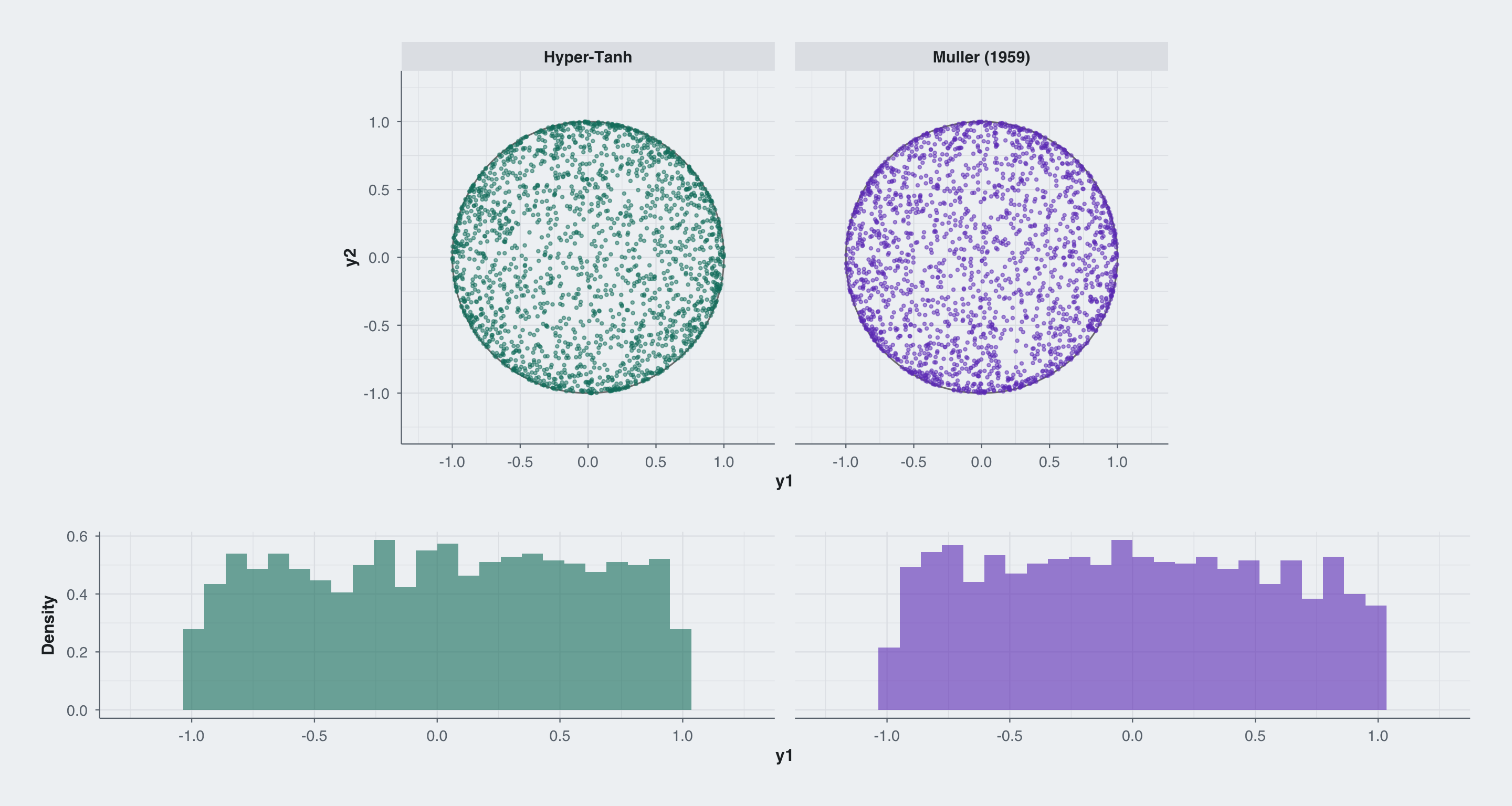
Experiment A: Uniformity Check
I generate 2,000 points on a 3D sphere (\(S^2\)) using both methods and verify that they cover the projected disk uniformly.
Code
set.seed(42)N <-2000df_muller <-generate_muller(N)df_ht <-generate_hypertanh_uniform(N)colnames(df_muller)[1:2] <-c("y1", "y2")colnames(df_ht)[1:2] <-c("y1", "y2")df_all <-rbind(df_muller, df_ht)# X-axis limits: sphere diameter (2) should be 80% of total width# So total width = 2 / 0.8 = 2.5, meaning xlim = c(-1.25, 1.25)xlims <-c(-1.25, 1.25)# Split data by method for individual plotsdf_ht_only <- df_all[df_all$Method =="Hyper-Tanh", ]df_muller_only <- df_all[df_all$Method =="Muller (1959)", ]# Use facet_grid for proper alignment# Reshape data for combined plotdf_scatter <- df_all %>%mutate(plot_type ="Isotropy")df_hist <- df_all %>%mutate(plot_type ="Marginal")# Scatter plot with facetsp_scatter <-ggplot(df_all, aes(x=y1, y=y2)) +annotate("path", x=cos(seq(0,2*pi,0.01)), y=sin(seq(0,2*pi,0.01)), color="grey50") +geom_point(aes(color=Method), size=0.8, alpha=0.5) +facet_wrap(~Method, nrow=1) +scale_color_manual(values=c(blog_colors$teal, blog_colors$purple)) +scale_x_continuous(limits=xlims, breaks=seq(-1, 1, 0.5)) +scale_y_continuous(limits=xlims, breaks=seq(-1, 1, 0.5)) +theme_blog() +labs(x="y1", y="y2") +theme(legend.position="none",aspect.ratio=1,panel.spacing =unit(1, "lines"))# Histogram with facetsp_hist <-ggplot(df_all, aes(x=y1, fill=Method)) +geom_histogram(aes(y=after_stat(density)), bins=30, alpha=0.6) +facet_wrap(~Method, nrow=1) +scale_fill_manual(values=c(blog_colors$teal, blog_colors$purple)) +scale_x_continuous(limits=xlims, breaks=seq(-1, 1, 0.5)) +theme_blog() +labs(x="y1", y="Density") +theme(legend.position="none",strip.text=element_blank(),panel.spacing =unit(1, "lines"))# Stack with patchworkp_scatter / p_hist +plot_layout(heights =c(1, 0.5))
Result: The Hyper-Tanh parameterization, when sampled with the correct Jacobian prior, is indistinguishable from Muller’s method. It is perfectly uniform.
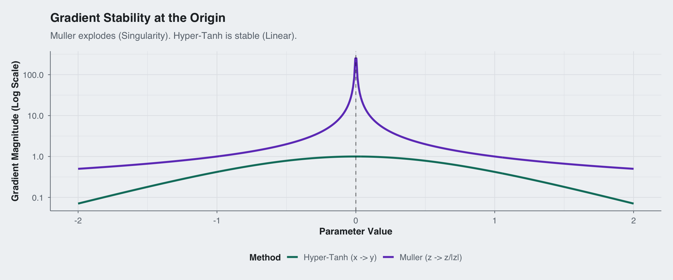
Experiment B: Gradient Stability (The “y=0” Singularity)
Here I calculate the magnitude of the gradient \(\left\| \frac{d\mathbf{y}}{dp} \right\|\) as the parameter \(p\) passes through the origin.
Result: The Hyper-Tanh Peel eliminates the topological singularity. The sampler can pass through the origin without experiencing infinite forces.
5. Stan Implementation
Copy this block directly into your Stan program.
functions {/** * Maps unconstrained R^(K-1) vector x to Unit Vector S^(K-1). * * @param x Unconstrained vector of length K-1 * @param K Dimension of the embedding space (output vector size) * @return Unit vector of length K */vectorhyper_tanh_to_unit_jacobian(vector x, int K) {vector[K] y;real r =1.0;for (i in1:K -2) {real val = x[i]; y[i] = r *tanh(val);real cosh_val =cosh(val); r = r *inv(cosh_val);real power = K - i; jacobian+=-power *log(cosh_val); }real last_x = x[K-1];jacobian+=log(2.0) -log1p(square(last_x));real denom =1.0+square(last_x); y[K-1] = r * (1.0-square(last_x)) / denom; y[K] = r * (2.0* last_x) / denom;return y; }}data {int<lower=2> K;}parameters {vector[K -1] x_raw; // Unconstrained}transformed parameters {vector[K] mu =hyper_tanh_to_unit_jacobian(x_raw, K);}model {// uniform on the sphere}
6. Conclusion
The hyper-tanh peel parameterization offers a robust alternative to Muller (1959)’s method for Bayesian modeling. It uses exactly \(K-1\) parameters, avoids the singularity at the origin by mapping from the pole, and might offer some interesting priors on the pullback.
References
Muller, Mervin E. 1959. “A Note on a Method for Generating Points Uniformly on n-Dimensional Spheres.”Commun. ACM 2 (4): 19–20. https://doi.org/10.1145/377939.377946.