Quantile regressions are relatively new in the Bayesian literature first appearing in Yu and Moyeed (2001) who described an asymmetric Laplace distribution to estimate the conditional quantiles. This post is going to show the asymmetric Laplace and the augmented version. In part II I will show the score likelihood method.

The asymmetric Laplace distribution is given as

\[ \operatorname{ALD}(Y \mid x, \beta) = \frac{\tau^n (1 - \tau)^n}{\sigma^n}\exp \bigg( -\frac{\sum_{i=1}^n \rho_\tau (y_i - x_i^{\top}\beta)}{\sigma} \bigg) \]

where

\[ \rho_\tau(u) = \frac{|u| + (2\tau - 1)u}{2} \]

We may write this in Stan as

Show the code

functions{
real q_loss(real q, vector u){
  return 0.5 * sum(abs(u) + (2 * q - 1) * u);
}

real ald_lpdf(vector y, real q, real sigma, vector q_est){
  int N = num_elements(y);
  
  return N * (log(q) + log1m(q) - log(sigma)) - q_loss(q, y - q_est) / sigma;
}
}
data {
  int N;                   // Number of observation
  int P;                   // Number of predictors
  real<lower=0, upper=1> q;
  vector[N] y;             // Response variable sorted
  matrix[N, P] x;
}
parameters {
  vector[P] beta;
  real<lower=0> sigma;
}
model {
  beta ~ normal(0, 4);
  sigma ~ exponential(1);
  y ~ ald(q, sigma, x * beta);
}

Let’s compare the 5th percentile to the Brq R package

Show the code

library(Brq)
data("ImmunogG")
out_asym_laplace <- asymetric_laplace$sample(
  data = list(N = nrow(ImmunogG),
              P = 3,
              q = 0.05,
              y = ImmunogG$IgG,
              x = as.matrix(data.frame(alpha = 1, x = ImmunogG$Age, xsq = ImmunogG$Age^2))),
  seed = 12123123, 
  parallel_chains = 4,
  iter_warmup = 500,
  iter_sampling = 500,
    refresh = 0,
  show_messages = FALSE
)

Running MCMC with 4 parallel chains...

Chain 1 finished in 0.5 seconds.
Chain 3 finished in 0.5 seconds.
Chain 4 finished in 0.5 seconds.
Chain 2 finished in 0.6 seconds.

All 4 chains finished successfully.
Mean chain execution time: 0.5 seconds.
Total execution time: 0.7 seconds.

Show the code

out_asym_laplace$summary()

# A tibble: 5 × 10
  variable     mean   median      sd     mad       q5      q95  rhat ess_bulk
  <chr>       <dbl>    <dbl>   <dbl>   <dbl>    <dbl>    <dbl> <dbl>    <dbl>
1 lp__     -670.    -670.    1.50    1.24    -673.    -669.     1.01     585.
2 beta[1]     0.587    0.601 0.246   0.271      0.179    0.962  1.02     385.
3 beta[2]     1.31     1.31  0.199   0.210      1.01     1.64   1.02     336.
4 beta[3]    -0.156   -0.155 0.0338  0.0333    -0.212   -0.104  1.01     373.
5 sigma       0.165    0.165 0.00958 0.00897    0.149    0.181  1.01     645.
# … with 1 more variable: ess_tail <dbl>

Show the code

y = ImmunogG$IgG
x = ImmunogG$Age
X=cbind(x, x^2)
fit = Brq(y ~ X , tau= 0.05,runs= 2000, burn=1000)
print(summary(fit))

Call:
Brq.formula(formula = y ~ X, tau = 0.05, runs = 2000, burn = 1000)

tau:[1] 0.05

            Estimate L.CredIntv  U.CredIntv
Intercept  0.6285948  0.1193195  1.04185440
Xx         1.2928087  0.8984968  1.67267316
X         -0.1541316 -0.2265564 -0.08528427

Using the covariates for extra information

In Lee, Chakraborty, and Su (2022) they detail a Bayesian approach to the envelope quantile regression. In all honesty, I briefly skimmed the paper and gathered that by adding a regression on the covariates and using this information in the asymmetric Laplace can help identification. This isn’t a recreation of their method but a quick detour to see if a simplified version of what they do increases ESS.

The idea is that we use the variability in the covariance of the regressors to help identify the coefficients on the ALD regression. I now have to separate out the intercept into \(\alpha\).

Show the code

functions{
real q_loss(real q, vector u){
  return 0.5 * sum(abs(u) + (2 * q - 1) * u);
}

real ald_lpdf(vector y, real q, real sigma, vector q_est){
  int N = num_elements(y);
  
  return N * (log(q) + log1m(q) - log(sigma)) - q_loss(q, y - q_est) / sigma;
}
}
data {
  int N;                   // Number of observation
  int P;                   // Number of predictors
  real<lower=0, upper=1> q;
  vector[N] y;             // Response variable sorted
  matrix[N, P] x;
}
transformed data {
  array[N] vector[P] X;
  
  for (i in 1:P) {
    X[:, i] = to_array_1d(x[:, i]);
  }
}
parameters {
  vector[P] eta;
  real<lower=0> sigma;
  vector[P] mu;
  cholesky_factor_corr[P] L;
  vector<lower=0>[P] gamma;
  real alpha;
}
transformed parameters {
  vector[P] beta = eta .* gamma;
}
model {
  eta ~ normal(0, 4);
  sigma ~ exponential(1);
  y ~ ald(q, sigma, alpha + x * beta);
  alpha ~ normal(0, 4);
  
  gamma ~ exponential(1);
  mu ~ normal(0, 4);

  X ~ multi_normal_cholesky(mu, diag_pre_multiply(gamma, L));
}

Let’s fit the model.

Show the code

out_envelope <- asymetric_laplace_envelope$sample(
  data = list(N = nrow(ImmunogG),
              P = 2,
              q = 0.05,
              y = ImmunogG$IgG,
              x = as.matrix(data.frame(x = ImmunogG$Age, xsq = ImmunogG$Age^2))),
  seed = 12123123, 
  parallel_chains = 4,
  iter_warmup = 500,
  iter_sampling = 500,
    refresh = 0,
  show_messages = FALSE
)

Running MCMC with 4 parallel chains...

Chain 1 finished in 10.2 seconds.
Chain 3 finished in 10.3 seconds.
Chain 2 finished in 10.6 seconds.
Chain 4 finished in 11.7 seconds.

All 4 chains finished successfully.
Mean chain execution time: 10.7 seconds.
Total execution time: 11.8 seconds.

Show the code

out_envelope$summary(c("alpha", "beta", "sigma"))

# A tibble: 4 × 10
  variable   mean median      sd     mad     q5    q95  rhat ess_bulk ess_tail
  <chr>     <dbl>  <dbl>   <dbl>   <dbl>  <dbl>  <dbl> <dbl>    <dbl>    <dbl>
1 alpha     0.600  0.626 0.244   0.258    0.182  0.955  1.01     662.    1022.
2 beta[1]   1.31   1.30  0.200   0.201    1.01   1.63   1.01     694.     845.
3 beta[2]  -0.155 -0.153 0.0348  0.0323  -0.216 -0.105  1.00     799.    1074.
4 sigma     0.166  0.165 0.00994 0.00953  0.150  0.182  1.00    1374.    1194.

Slightly different estimates, higher ESS, slower to fit, but lower standard deviations! Neat.

Scale-mixture representation

The above may also be written as a mixture of exponential and normal distributions. Letting

\[ \begin{aligned} z_i &\sim \operatorname{Exp}(1) \\ \sigma &\sim \operatorname{Exp}(1) \\ y_i &\sim \mathcal{N}(x_i^{\top}\beta_p + \sigma \theta z_i,\, \tau \sigma \sqrt{z_i}) \end{aligned} \] where

\[ \begin{aligned} \theta &= \frac{1 - 2 q}{q (1 - q)} \\ \tau &= \sqrt{\frac{2}{q(1 -q)}} \end{aligned} \]

The following Stan model implements the augmented approach.

Show the code

data {
  int N;                   // Number of observation
  int P;                   // Number of predictors
  real<lower=0, upper=1> q;
  vector[N] y;             // Response variable sorted
  matrix[N, P] x;
}
transformed data {
  real theta = (1 - 2 * q) / (q * (1 - q));
  real tau = sqrt(2 / (q * (1 - q)));
}
parameters {
  vector[P] beta;
  vector<lower=0>[N] z;
  real<lower=0> sigma;
}
model {
  beta ~ normal(0, 2);
  sigma ~ exponential(1);
  
  // Data Augmentation
  z ~ exponential(1);
  y ~ normal(x * beta + sigma * theta * z, tau * sqrt(z) * sigma);
}

Let’s fit the model

Show the code

out_aug_laplace <- augmented_laplace$sample(
  data = list(N = nrow(ImmunogG),
              P = 3,
              q = 0.05,
              y = ImmunogG$IgG,
              x = as.matrix(data.frame(alpha = 1, x = ImmunogG$Age, xsq = ImmunogG$Age^2))),
  seed = 12123123, 
  parallel_chains = 4,
  iter_warmup = 500,
  iter_sampling = 500,
    refresh = 0,
  show_messages = FALSE
)

Running MCMC with 4 parallel chains...

Chain 1 finished in 3.8 seconds.
Chain 3 finished in 3.8 seconds.
Chain 2 finished in 4.2 seconds.
Chain 4 finished in 4.3 seconds.

All 4 chains finished successfully.
Mean chain execution time: 4.0 seconds.
Total execution time: 4.3 seconds.

Warning: 77 of 2000 (4.0%) transitions ended with a divergence.
See https://mc-stan.org/misc/warnings for details.

Show the code

out_aug_laplace$summary(c("beta"))

# A tibble: 3 × 10
  variable   mean median     sd    mad     q5     q95  rhat ess_bulk ess_tail
  <chr>     <dbl>  <dbl>  <dbl>  <dbl>  <dbl>   <dbl> <dbl>    <dbl>    <dbl>
1 beta[1]   0.589  0.596 0.249  0.264   0.169  0.982   1.01     443.     733.
2 beta[2]   1.31   1.32  0.210  0.201   0.953  1.64    1.01     397.     505.
3 beta[3]  -0.155 -0.155 0.0354 0.0321 -0.216 -0.0973  1.01     394.     522.

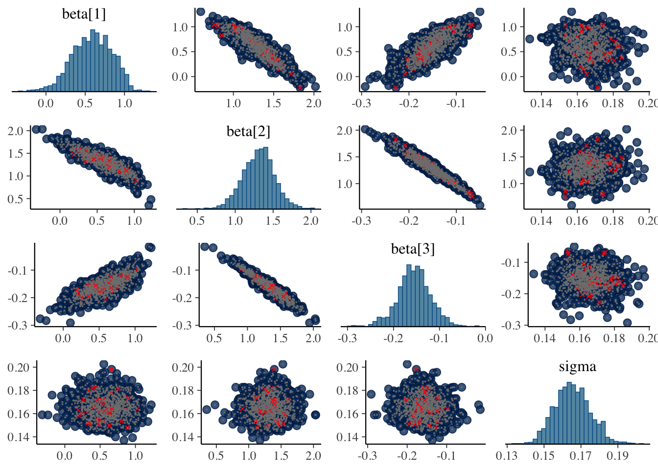
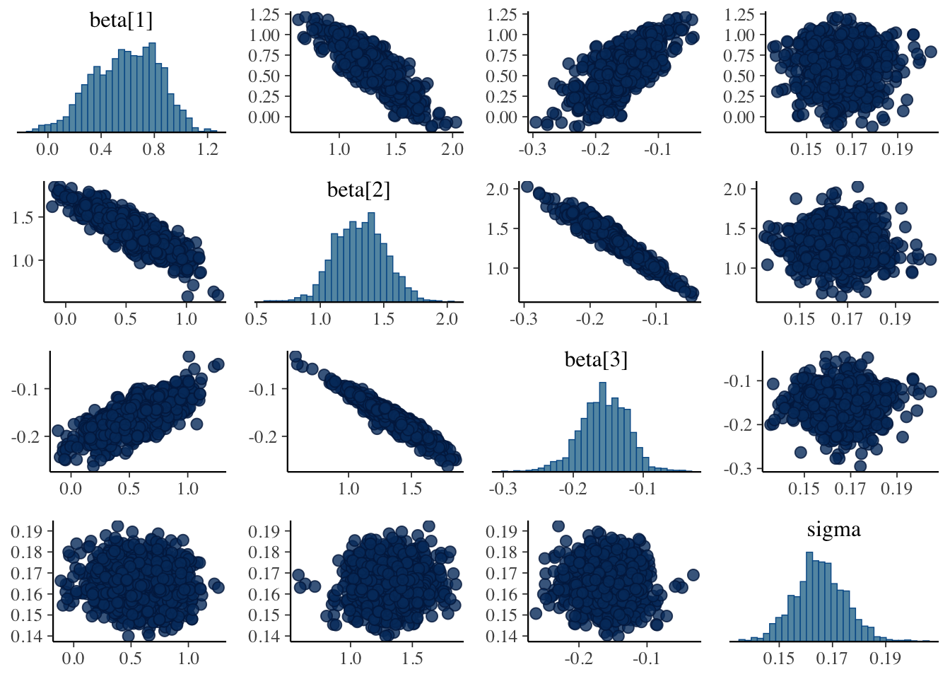
Ouch! Divergences. Although the parameter estimates look comparable. Let’s inspect the pairs plots between the augmented version and the asymmetric Laplace.

Show the code

library(bayesplot)

This is bayesplot version 1.9.0

- Online documentation and vignettes at mc-stan.org/bayesplot

- bayesplot theme set to bayesplot::theme_default()

   * Does _not_ affect other ggplot2 plots

   * See ?bayesplot_theme_set for details on theme setting

Show the code

np_aug_laplace <- nuts_params(out_aug_laplace)
np_asym_laplace <- nuts_params(out_asym_laplace)
mcmc_pairs(out_aug_laplace$draws(c("beta", "sigma")), np = np_aug_laplace)

Show the code

mcmc_pairs(out_asym_laplace$draws(c("beta", "sigma")), np = np_asym_laplace)

The pairs plots don’t appear to show the divergence originating be due to beta or sigma. It’s most likely the augmentation variables z. As I’m up for time on this, I’d be curious to test out alternative specifications or see if anyone has encountered these issues with the augmented version and found a solution.

Try Student T

Warning

The Student T won’t result in the same posterior and is likely not ALD. However, it approaches a normal distribution with increasing \(\nu\).

Let’s use the student_t with \(\nu = 30\)

Show the code

data {
  int N;                   // Number of observation
  int P;                   // Number of predictors
  real<lower=0, upper=1> q;
  vector[N] y;             // Response variable sorted
  matrix[N, P] x;
}
transformed data {
  real theta = (1 - 2 * q) / (q * (1 - q));
  real tau = sqrt(2 / (q * (1 - q)));
}
parameters {
  vector[P] beta;
  vector<lower=0>[N] z;
  real<lower=0> sigma;
}
model {
  beta ~ normal(0, 2);
  sigma ~ exponential(1);
  
  // Data Augmentation
  z ~ exponential(1);
  y ~ student_t(30, x * beta + sigma * theta * z, tau * sqrt(z) * sigma);
}

Let’s fit the same model

Show the code

out_student_aug_laplace <- student_augmented_laplace$sample(
  data = list(N = nrow(ImmunogG),
              P = 3,
              q = 0.05,
              y = ImmunogG$IgG,
              x = as.matrix(data.frame(alpha = 1, x = ImmunogG$Age, xsq = ImmunogG$Age^2))),
  seed = 12123123, 
  parallel_chains = 4,
  iter_warmup = 500,
  iter_sampling = 500,
    refresh = 0,
  show_messages = FALSE
)

Running MCMC with 4 parallel chains...

Chain 3 finished in 4.4 seconds.
Chain 1 finished in 4.5 seconds.
Chain 4 finished in 4.5 seconds.
Chain 2 finished in 4.8 seconds.

All 4 chains finished successfully.
Mean chain execution time: 4.6 seconds.
Total execution time: 4.9 seconds.

Show the code

out_student_aug_laplace$summary(c("beta"))

# A tibble: 3 × 10
  variable   mean median     sd    mad     q5    q95  rhat ess_bulk ess_tail
  <chr>     <dbl>  <dbl>  <dbl>  <dbl>  <dbl>  <dbl> <dbl>    <dbl>    <dbl>
1 beta[1]   0.621  0.650 0.231  0.228   0.207  0.961  1.01     442.     682.
2 beta[2]   1.33   1.32  0.169  0.162   1.06   1.62   1.01     448.     803.
3 beta[3]  -0.155 -0.154 0.0271 0.0258 -0.201 -0.111  1.01     487.     797.

Great no divergences!

Conclusion

For the next post, we’ll take a look at an approximate likelihood using the data which asymptotically approaches the true likelihood with more data.

References

Lee, Minji, Saptarshi Chakraborty, and Zhihua Su. 2022. “A Bayesian Approach to Envelope Quantile Regression.” Statistica Sinica, January. https://doi.org/10.5705/ss.202020.0109.

Yu, Keming, and Rana A. Moyeed. 2001. “Bayesian Quantile Regression.” Statistics & Probability Letters 54 (4): 437–47. https://doi.org/https://doi.org/10.1016/S0167-7152(01)00124-9.