Bounded Correlation Matrices: Sign Constraints, Finite Boxes, and Exact Values

stan
correlation
parameterizations
Author

Sean Pinkney

Published

August 8, 2026

1. From Structural Zeros to Bounds

My previous post used a triangular basis to sample correlation matrices with exact structural zeros. Given the preceding Cholesky rows, each zero is a homogeneous linear constraint on the current row, and the zero vector remains an admissible row completion after every valid prefix. Here I ask how much of that construction carries over to prescribed signs, finite cell-specific intervals, and exact nonzero values.

I ended up with three different cases.

  1. Prescribed signs admit a smooth triangular transform. Zeros define subspaces; signs define cones. Replacing the free coordinates in each Cholesky row by coordinates inside the requested sign cone gives a bijection onto the interior of the sign-constrained correlation space. Section 3 gives the row-wise inverse.

  2. Finite boxes do not fit the same homogeneous construction. A box such as \(0.2 < \Omega_{21} < 0.5\) is not scale invariant, so the linear zero basis does not represent it. For this case, I use rays from a strictly feasible anchor. Section 4 shows that the resulting map covers the interior of the box–elliptope intersection, apart from the anchor itself. Its active boundary can change with direction and create gradient kinks.

  3. An exact nonzero value is an affine equality. A translated version of the zero-row construction exists, but its available radius depends on earlier correlations and can disappear after an otherwise valid prefix. For general fixed-value patterns, I instead remove the fixed coordinates from the global anchor-ray map.

Throughout, the LKJ shape \(\eta>0\) is fixed. The target is an LKJ density (Lewandowski et al. 2009) restricted to the requested ordinary-correlation region,

\[\pi(\Omega) \propto \det(\Omega)^{\eta-1} \mathbf 1\{\ell_{ij}<\Omega_{ij}<u_{ij}\},\]

with respect to Lebesgue measure on the free lower-triangular correlations. For positive-width free bounds, endpoint faces have measure zero, so open and closed interval notation induce the same continuous distribution.

When some correlations are fixed exactly, I instead define the density with respect to the remaining free ordinary-correlation coordinates. This is a lower-dimensional target, not an unnormalized positive-width indicator with equal endpoints. Any shrinking-interval argument must keep its width-dependent normalizing constant.

The general look-ahead C-vine implementation and my earlier entry-wise Cholesky construction (Pinkney 2024) provide sequential ways to target bounded densities, although a later feasible interval can be empty. Here I focus on transforms that make global feasibility explicit, so a sequential construction does not encounter a nonlocal boundary late.

2. Why the Zero-Basis Construction Does Not Extend Directly

Write \(\Omega=LL'\) and consider row \(i\). Let

\[B=L_{1:(i-1),1:(i-1)}, \qquad v=L_{i,1:(i-1)}', \qquad c=\Omega_{i,1:(i-1)}'.\]

The ordinary correlations in the row satisfy

\[c=Bv,\]

and positive definiteness requires \(v'v<1\) so that \(L_{ii}=\sqrt{1-v'v}>0\). Therefore the feasible set for \(c\) given the previous rows is the Schur ellipsoid

\[\mathcal E_B=\{c:c'(BB')^{-1}c<1\}.\]

An exact zero selects a linear slice through this ellipsoid. To see what this buys, let \(d=i-1\) and suppose that the entries indexed by \(Z=\{j_1,\ldots,j_m\}\subseteq\{1,\ldots,d\}\) are fixed to zero. Define the coordinate-selection matrix \(P_Z\in\mathbb R^{m\times d}\) by taking its \(r\)th row to be the transpose of the \(j_r\)th standard basis vector, \(e_{j_r}'\). Thus, for any \(x\in\mathbb R^d\),

\[P_Zx=(x_{j_1},\ldots,x_{j_m})'.\]

Multiplication by \(P_Z\) simply extracts the coordinates indexed by \(Z\). The \(m\) zero constraints can therefore be collected as

\[P_Zc=P_ZBv=0.\]

These are homogeneous linear equations in \(v\). The leading Cholesky block \(B\) is nonsingular, so the selected rows \(P_ZB\) are linearly independent and have rank \(m\). The constraints therefore remove exactly \(m\) degrees of freedom and leave the \((d-m)\)-dimensional subspace \(\ker(P_ZB)\). The orthogonal-complement construction of Axen (2023) and the triangular construction from my previous post span this same nullspace, but they choose its basis differently. The former computes a complement to the constrained rows. The latter ties the basis to the free entries of the Cholesky row: for each free coordinate, it sets that coordinate to one and the other free coordinates to zero, solves the constrained coordinates by back-substitution, and then orthonormalizes the resulting basis.

If \(Q\) denotes either orthonormal basis, write \(v=Qz\), so that \(v'v=z'z\). One can then sample \(z\) in the open unit ball in \(\mathbb R^{d-m}\) and set

\[L_{ii}=\sqrt{1-z'z}.\]

The pair \((z,L_{ii})\) lies on a \((d-m)\)-dimensional unit hemisphere, and multiplication by \(Q\) lifts \(z\) into the original off-diagonal coordinates \(v\). Every lifted row satisfies the zero constraints automatically, and every feasible row in the constrained subspace has such a representation. Thus the basis construction does more than enforce the zeros: it removes exactly the coordinates that the equalities have made redundant while retaining the usual hemisphere parameterization of a unit-norm Cholesky row.

Bounds instead produce

\[\mathcal E_B \cap \{c:\ell<c<u\},\]

an ellipsoid intersected with slabs. Assume here that every interval has positive width. Both the Schur ellipsoid and the open box \(\{c:\ell<c<u\}\) are open subsets of \(\mathbb R^d\), so whenever their intersection is nonempty, every feasible point has a sufficiently small \(d\)-dimensional neighborhood that remains feasible. The bounds can truncate the allowable range along a direction, but they do not remove a local degree of freedom as an equality does.

They also change the boundary geometry. In the closure of the feasible set, a bound that is reached before the positive-definite boundary contributes a flat codimension-one face \(c_j=\ell_j\) or \(c_j=u_j\). Several active bounds can meet in edges or corners, while the condition \(c'(BB')^{-1}c=1\) contributes the curved ellipsoid boundary. Which piece is encountered first depends on the point and direction. There is therefore no fixed lower-dimensional subspace whose basis encodes the interval constraints: removing a basis column handles an equality, whereas an inequality must retain the coordinate and control how far it may move. The column-removal step used for exact zeros consequently does not impose these bounds by itself. Clipping correlations after the transform would change the induced density and can also break positive definiteness.

Code
library(ggplot2)
source("../../R/theme_blog.R")

schur_constraint_plot <- local({
  previous_block <- matrix(
    c(
      1.0, 0.5, 0.5,
      0.5, 1.0, 0.5,
      0.5, 0.5, 1.0
    ),
    nrow = 3,
    byrow = TRUE
  )
  previous_cholesky <- chol(previous_block)

  lower_bound <- 0.55
  upper_bound <- 0.85
  fixed_nonzero <- 0.70
  lower_free_radius <- sqrt(1 - lower_bound^2)
  upper_free_radius <- sqrt(1 - upper_bound^2)
  fixed_free_radius <- sqrt(1 - fixed_nonzero^2)

  zero_panel <- paste(
    "Exact zero:  c₁ = 0",
    "2D linear section",
    "0² + free² < 1;  free radius = 1.00",
    sep = "\n"
  )
  bound_panel <- paste(
    "Finite bound:  0.55 < c₁ < 0.85",
    "3D off-origin volume",
    sprintf(
      "free radius varies: %.2f down to %.2f",
      lower_free_radius,
      upper_free_radius
    ),
    sep = "\n"
  )
  nonzero_panel <- paste(
    "Exact nonzero:  c₁ = 0.70",
    "2D affine section",
    sprintf(
      "0.70² + free² < 1;  free radius = %.2f",
      fixed_free_radius
    ),
    sep = "\n"
  )
  panel_levels <- c(zero_panel, bound_panel, nonzero_panel)

  stopifnot(
    min(eigen(
      previous_block,
      symmetric = TRUE,
      only.values = TRUE
    )$values) > 0,
    -1 < lower_bound,
    lower_bound < upper_bound,
    upper_bound < 1,
    0 < fixed_nonzero,
    fixed_nonzero < 1
  )

  azimuth <- 72 * pi / 180
  elevation <- 30 * pi / 180
  roll <- -14 * pi / 180
  right <- c(-sin(azimuth), cos(azimuth), 0)
  up <- c(
    -sin(elevation) * cos(azimuth),
    -sin(elevation) * sin(azimuth),
    cos(elevation)
  )

  project_3d <- function(points) {
    projected <- as.matrix(points) %*% cbind(right, up)
    data.frame(
      x = cos(roll) * projected[, 1] -
        sin(roll) * projected[, 2],
      y = sin(roll) * projected[, 1] +
        cos(roll) * projected[, 2]
    )
  }

  ellipsoid_section <- function(value, n = 481) {
    angle <- seq(0, 2 * pi, length.out = n)
    radius <- sqrt(1 - value^2)
    sphere_section <- cbind(
      value,
      radius * cos(angle),
      radius * sin(angle)
    )
    sphere_section %*% previous_cholesky
  }

  section_check <- ellipsoid_section(fixed_nonzero)
  previous_precision <- solve(previous_block)
  stopifnot(
    max(abs(section_check[, 1] - fixed_nonzero)) < 1e-12,
    max(abs(
      rowSums(
        (section_check %*% previous_precision) * section_check
      ) - 1
    )) < 1e-10
  )

  ellipsoid_rail <- function(angle, from, to, n = 241) {
    first <- seq(from, to, length.out = n)
    radius <- sqrt(1 - first^2)
    sphere_rail <- cbind(
      first,
      radius * cos(angle),
      radius * sin(angle)
    )
    sphere_rail %*% previous_cholesky
  }

  with_panel <- function(data, panel, group = NULL) {
    data$panel <- factor(panel, levels = panel_levels)
    if (!is.null(group)) {
      data$group <- paste(panel, group, sep = "::")
    }
    data
  }

  # Common ellipsoid silhouette.
  surface_grid <- expand.grid(
    first = seq(-0.999, 0.999, length.out = 61),
    angle = seq(0, 2 * pi, length.out = 121)
  )
  surface_radius <- sqrt(1 - surface_grid$first^2)
  surface_sphere <- cbind(
    surface_grid$first,
    surface_radius * cos(surface_grid$angle),
    surface_radius * sin(surface_grid$angle)
  )
  surface_projection <- project_3d(
    surface_sphere %*% previous_cholesky
  )
  silhouette_one <- surface_projection[
    chull(surface_projection$x, surface_projection$y),
  ]
  silhouette <- do.call(rbind, lapply(panel_levels, function(panel) {
    with_panel(silhouette_one, panel, "ellipsoid")
  }))

  # Sparse common wireframe.
  wire_parts <- list()
  wire_id <- 1
  for (value in seq(-0.8, 0.8, by = 0.2)) {
    wire_parts[[wire_id]] <- cbind(
      project_3d(ellipsoid_section(value)),
      wire_group = paste0("ring", wire_id)
    )
    wire_id <- wire_id + 1
  }
  for (angle in seq(0, 330, by = 30) * pi / 180) {
    wire_parts[[wire_id]] <- cbind(
      project_3d(ellipsoid_rail(angle, -0.999, 0.999)),
      wire_group = paste0("rail", wire_id)
    )
    wire_id <- wire_id + 1
  }
  wire_one <- do.call(rbind, wire_parts)
  ellipsoid_wire <- do.call(rbind, lapply(panel_levels, function(panel) {
    with_panel(wire_one, panel, wire_one$wire_group)
  }))

  zero_slice <- with_panel(
    project_3d(ellipsoid_section(0)),
    zero_panel,
    "zero"
  )
  nonzero_slice <- with_panel(
    project_3d(ellipsoid_section(fixed_nonzero)),
    nonzero_panel,
    "nonzero"
  )

  # The interval intersection: a projected silhouette, internal sections,
  # curved boundary rails, and the two planar endpoint faces.
  volume_grid <- expand.grid(
    first = seq(lower_bound, upper_bound, length.out = 81),
    angle = seq(0, 2 * pi, length.out = 181)
  )
  volume_radius <- sqrt(1 - volume_grid$first^2)
  volume_sphere <- cbind(
    volume_grid$first,
    volume_radius * cos(volume_grid$angle),
    volume_radius * sin(volume_grid$angle)
  )
  volume_projection <- project_3d(
    volume_sphere %*% previous_cholesky
  )
  volume_silhouette <- with_panel(
    volume_projection[
      chull(volume_projection$x, volume_projection$y),
    ],
    bound_panel,
    "volume"
  )

  internal_values <- seq(
    lower_bound,
    upper_bound,
    length.out = 7
  )[2:6]
  bound_sections <- do.call(rbind, lapply(
    seq_along(internal_values),
    function(index) {
      with_panel(
        project_3d(ellipsoid_section(internal_values[index])),
        bound_panel,
        paste0("section", index)
      )
    }
  ))
  bound_rails <- do.call(rbind, lapply(
    seq_along(seq(0, 330, by = 30)),
    function(index) {
      angle <- seq(0, 330, by = 30)[index] * pi / 180
      with_panel(
        project_3d(ellipsoid_rail(
          angle,
          lower_bound,
          upper_bound
        )),
        bound_panel,
        paste0("bound_rail", index)
      )
    }
  ))
  bound_faces <- rbind(
    with_panel(
      project_3d(ellipsoid_section(lower_bound)),
      bound_panel,
      "lower_face"
    ),
    with_panel(
      project_3d(ellipsoid_section(upper_bound)),
      bound_panel,
      "upper_face"
    )
  )

  # A common c1 axis and origin make central versus affine obvious.
  c1_axis_3d <- rbind(c(-1.08, 0, 0), c(1.08, 0, 0))
  c1_axis_projected <- project_3d(c1_axis_3d)
  c1_axis <- do.call(rbind, lapply(panel_levels, function(panel) {
    data.frame(
      x = c1_axis_projected$x[1],
      y = c1_axis_projected$y[1],
      xend = c1_axis_projected$x[2],
      yend = c1_axis_projected$y[2],
      panel = factor(panel, levels = panel_levels)
    )
  }))
  c1_label <- do.call(rbind, lapply(panel_levels, function(panel) {
    data.frame(
      x = c1_axis_projected$x[2],
      y = c1_axis_projected$y[2],
      label = "c[1]",
      panel = factor(panel, levels = panel_levels)
    )
  }))
  origin_projection <- project_3d(matrix(c(0, 0, 0), nrow = 1))
  origins <- data.frame(
    x = origin_projection$x,
    y = origin_projection$y,
    panel = factor(panel_levels, levels = panel_levels)
  )
  origin_labels <- transform(
    origins,
    x = x + 0.05,
    y = y + 0.055,
    label = "0"
  )

  nonzero_center_3d <- c(
    fixed_nonzero,
    0.5 * fixed_nonzero,
    0.5 * fixed_nonzero
  )
  nonzero_center <- project_3d(matrix(nonzero_center_3d, nrow = 1))
  offset_segment <- data.frame(
    x = origin_projection$x,
    y = origin_projection$y,
    xend = nonzero_center$x,
    yend = nonzero_center$y,
    panel = factor(nonzero_panel, levels = panel_levels)
  )

  # In Cholesky coordinates, fixing the first coordinate to q leaves
  # v_2^2 + v_3^2 < 1 - q^2. Draw one transformed radius in each
  # section so the spent and remaining parts of that budget are visible.
  free_radius_segment <- function(value, panel) {
    radius <- sqrt(1 - value^2)
    points <- rbind(
      c(value, 0, 0),
      c(value, 0, radius)
    ) %*% previous_cholesky
    projected <- project_3d(points)
    data.frame(
      x = projected$x[1],
      y = projected$y[1],
      xend = projected$x[2],
      yend = projected$y[2],
      panel = factor(panel, levels = panel_levels)
    )
  }

  zero_radius_segment <- free_radius_segment(0, zero_panel)
  bound_radius_segments <- rbind(
    transform(
      free_radius_segment(lower_bound, bound_panel),
      face = "lower"
    ),
    transform(
      free_radius_segment(upper_bound, bound_panel),
      face = "upper"
    )
  )
  nonzero_radius_segment <- free_radius_segment(
    fixed_nonzero,
    nonzero_panel
  )

  radius_target <- function(segment, fraction = 0.62) {
    c(
      x = segment$x + fraction * (segment$xend - segment$x),
      y = segment$y + fraction * (segment$yend - segment$y)
    )
  }
  callout_targets <- rbind(
    radius_target(zero_radius_segment),
    radius_target(subset(bound_radius_segments, face == "lower")),
    radius_target(subset(bound_radius_segments, face == "upper")),
    radius_target(nonzero_radius_segment)
  )
  free_radius_arrows <- data.frame(
    arrow_x = c(0.40, -0.10, -0.26, -0.37),
    arrow_y = rep(0.84, 4),
    xend = callout_targets[, "x"],
    yend = callout_targets[, "y"],
    constraint = factor(
      c("zero", "bound", "bound", "nonzero"),
      levels = c("zero", "bound", "nonzero")
    ),
    panel = factor(
      c(zero_panel, bound_panel, bound_panel, nonzero_panel),
      levels = panel_levels
    )
  )
  free_radius_labels <- data.frame(
    label_x = c(0.40, -0.18, -0.37),
    label_y = rep(0.91, 3),
    constraint = factor(
      c("zero", "bound", "nonzero"),
      levels = c("zero", "bound", "nonzero")
    ),
    panel = factor(panel_levels, levels = panel_levels),
    label = "free radius"
  )

  ggplot() +
    geom_polygon(
      data = silhouette,
      aes(x, y, group = group),
      fill = blog_colors$blue,
      color = NA,
      alpha = 0.055
    ) +
    geom_path(
      data = ellipsoid_wire,
      aes(x, y, group = group),
      color = blog_colors$blue,
      alpha = 0.07,
      linewidth = 0.35
    ) +
    geom_segment(
      data = c1_axis,
      aes(x = x, y = y, xend = xend, yend = yend),
      color = blog_colors$text_light,
      linetype = "22",
      linewidth = 0.55,
      arrow = grid::arrow(
        length = grid::unit(0.10, "cm"),
        type = "closed"
      )
    ) +
    geom_polygon(
      data = volume_silhouette,
      aes(x, y, group = group),
      fill = blog_colors$teal,
      color = NA,
      alpha = 0.045
    ) +
    geom_path(
      data = bound_sections,
      aes(x, y, group = group),
      color = blog_colors$teal,
      alpha = 0.24,
      linewidth = 0.35
    ) +
    geom_path(
      data = bound_rails,
      aes(x, y, group = group),
      color = blog_colors$teal,
      alpha = 0.48,
      linewidth = 0.45
    ) +
    geom_polygon(
      data = subset(bound_faces, grepl("lower_face", group)),
      aes(x, y, group = group),
      fill = blog_colors$teal,
      color = blog_colors$teal,
      alpha = 0.06,
      linetype = "22",
      linewidth = 0.9
    ) +
    geom_polygon(
      data = subset(bound_faces, grepl("upper_face", group)),
      aes(x, y, group = group),
      fill = blog_colors$teal,
      color = blog_colors$teal,
      alpha = 0.16,
      linewidth = 1.05
    ) +
    geom_polygon(
      data = zero_slice,
      aes(x, y, group = group),
      fill = blog_colors$purple,
      color = blog_colors$purple,
      alpha = 0.27,
      linewidth = 1.2
    ) +
    geom_polygon(
      data = nonzero_slice,
      aes(x, y, group = group),
      fill = blog_colors$gold,
      color = blog_colors$gold,
      alpha = 0.27,
      linewidth = 1.2
    ) +
    geom_path(
      data = ellipsoid_wire,
      aes(x, y, group = group),
      color = blog_colors$blue,
      alpha = 0.23,
      linewidth = 0.30
    ) +
    geom_segment(
      data = zero_radius_segment,
      aes(x = x, y = y, xend = xend, yend = yend),
      color = blog_colors$purple,
      linewidth = 1.05,
      arrow = grid::arrow(
        length = grid::unit(0.10, "cm"),
        type = "closed"
      )
    ) +
    geom_segment(
      data = bound_radius_segments,
      aes(x = x, y = y, xend = xend, yend = yend),
      color = blog_colors$teal,
      linewidth = 1.05,
      arrow = grid::arrow(
        length = grid::unit(0.10, "cm"),
        type = "closed"
      )
    ) +
    geom_segment(
      data = offset_segment,
      aes(x = x, y = y, xend = xend, yend = yend),
      color = blog_colors$gold,
      linetype = "22",
      linewidth = 0.95,
      arrow = grid::arrow(
        length = grid::unit(0.10, "cm"),
        type = "closed"
      )
    ) +
    geom_segment(
      data = nonzero_radius_segment,
      aes(x = x, y = y, xend = xend, yend = yend),
      color = blog_colors$gold,
      linewidth = 1.05,
      arrow = grid::arrow(
        length = grid::unit(0.10, "cm"),
        type = "closed"
      )
    ) +
    geom_point(
      data = origins,
      aes(x, y),
      shape = 21,
      fill = blog_colors$background,
      color = blog_colors$navy,
      size = 2.6,
      stroke = 0.9
    ) +
    geom_text(
      data = origin_labels,
      aes(x, y, label = label),
      color = blog_colors$navy,
      size = 3.0,
      hjust = 0,
      vjust = 0
    ) +
    geom_point(
      data = transform(
        nonzero_center,
        panel = factor(nonzero_panel, levels = panel_levels)
      ),
      aes(x, y),
      color = blog_colors$gold,
      size = 2.4
    ) +
    geom_curve(
      data = free_radius_arrows,
      aes(
        x = arrow_x,
        y = arrow_y,
        xend = xend,
        yend = yend,
        color = constraint
      ),
      curvature = 0.10,
      linewidth = 0.65,
      arrow = grid::arrow(
        length = grid::unit(0.10, "cm"),
        type = "closed"
      )
    ) +
    geom_text(
      data = free_radius_labels,
      aes(
        x = label_x,
        y = label_y,
        label = label,
        color = constraint
      ),
      fontface = "bold",
      size = 3.0
    ) +
    geom_text(
      data = c1_label,
      aes(x, y, label = label),
      parse = TRUE,
      color = blog_colors$text_light,
      hjust = 1.1,
      vjust = 1.1,
      size = 3.3
    ) +
    scale_color_manual(
      values = c(
        zero = blog_colors$purple,
        bound = blog_colors$teal,
        nonzero = blog_colors$gold
      ),
      guide = "none"
    ) +
    facet_wrap(~panel, nrow = 1) +
    coord_equal(
      xlim = c(-1.35, 1.35),
      ylim = c(-1.20, 1.25),
      expand = FALSE
    ) +
    theme_blog() +
    theme(
      panel.grid = element_blank(),
      panel.grid.major = element_blank(),
      panel.grid.minor = element_blank(),
      axis.title = element_blank(),
      axis.text = element_blank(),
      axis.ticks = element_blank(),
      axis.line = element_blank(),
      legend.position = "none",
      strip.text = element_text(size = 9.6, lineheight = 1.12)
    ) +
    labs(
      title = "Zero, Bound, and Nonzero Constraints Use the Row Budget Differently",
      subtitle = paste(
        "Cholesky-row budget:  q² + free² < 1.",
        "Fixing q leaves radius √(1 − q²); an interval makes that radius vary."
      )
    )
})

schur_constraint_plot
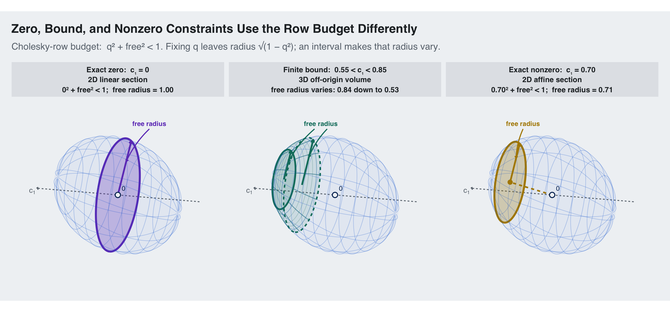
Figure 1: All three panels fix the leading \(3\times3\) block \(R\) and vary \(c=(\Omega_{4,1},\Omega_{4,2},\Omega_{4,3})\). In this example the first Cholesky-row coordinate equals \(c_1=q\), so positive definiteness requires \(q^2+v_2^2+v_3^2<1\). The colored spokes show the image of the remaining Cholesky radius \(\sqrt{1-q^2}\): it is \(1\) at zero, falls from \(0.84\) to \(0.53\) across the bounded interval, and is \(0.71\) at the exact value \(q=0.70\). Thus zero is a homogeneous section through the full radius, the bound retains three-dimensional volume but gives every section a different budget, and the nonzero equality is an affine section with \(0.49\) of the squared-norm budget already fixed. With several fixed values, the fixed share is generally \(\kappa=q^{\mathsf T}G^{-1}q\) and the remaining radius is \(\sqrt{1-\kappa}\); it can shrink to tangency or become infeasible. The ordinary-correlation intersections remain convex, so the difficulty is a completion boundary rather than disconnected target regions. Look-ahead propagates \([0,0]\), \([\ell,u]\), and \([q,q]\) through the same local \(3\times3\) projection.

3. The Smooth Triangular Sign Transform

Sign constraints retain one useful property: they are homogeneous. If \(c\) has the right signs, then \(a c\) has the same signs for every \(a>0\). Their directions form an orthant cone; the Schur ellipsoid truncates each ray at the positive-definite boundary.

Let \(s_j\in\{-1,+1\}\) be the requested sign of correlation \((i,j)\). Choose a smooth, strictly increasing bijection \(g:\mathbb R\to(0,\infty)\) with \(g'(y)>0\), and set

\[x_j=s_j\,g(y_j), \qquad g(y)>0.\]

The implementation uses the numerically stable softplus divided by \(2K\), which has these properties. The factor \(2K\) changes the scale near the default initialization but not the image \((0,\infty)\). Solve through the previous Cholesky triangle,

\[w=B^{-1}x, \qquad t=w'w,\]

then reuse the modified stereographic hemisphere map from Pinkney (2025),

\[a(t)=\frac{\sqrt{t+2}}{t+1}, \qquad v=a(t)w, \qquad L_{ii}=\frac{1}{t+1}.\]

The row has unit norm because

\[v'v+L_{ii}^2 =\frac{t(t+2)+1}{(t+1)^2}=1.\]

The corresponding ordinary correlations are

\[c=Bv=a(t)Bw=a(t)x.\]

Since \(a(t)>0\), every correlation has exactly the requested sign. In exact arithmetic, every finite raw vector therefore produces a positive-definite correlation matrix in the desired orthant without a feasibility check, projection, or rejection.

To check coverage conditional on the previous rows, take any \(c\) with the prescribed strict signs and \(q=c'(BB')^{-1}c<1\). Set \(v=B^{-1}c\). The inverse radial coordinate is unique:

\[t=\frac{1}{\sqrt{1-q}}-1.\]

Then \(w=v/a(t)\) and \(x=Bw=c/a(t)\). Because \(a(t)>0\), \(x\) has the same signs as \(c\), and \(g\) can be inverted coordinate by coordinate. Thus each admissible row has one finite raw preimage. Applying this inverse successively from row 2 through row \(K\) establishes the bijection for the complete matrix.

3.1 Jacobian

At fixed earlier rows, the determinants from \(x\mapsto w=B^{-1}x\) and \(v\mapsto c=Bv\) cancel. For \(d=i-1\), the row contribution with respect to the ordinary correlations is

\[\det\left\{\frac{\partial(a(t)w)}{\partial w}\right\} =a(t)^d\left\{1+2t\frac{a'(t)}{a(t)}\right\} =\frac{2(t+2)^{(d-2)/2}}{(1+t)^{d+1}},\]

where the first equality follows from the matrix determinant lemma. Including the coordinate-wise derivative of \(g\) gives

\[\log J_i =\sum_{j=1}^{d}\log g'(y_j) +\log 2 +\frac{d-2}{2}\log(t+2) -(d+1)\log(1+t).\]

The complete raw-to-free-correlation Jacobian is block triangular by rows, so the full log Jacobian is \(\sum_i\log J_i\). The Stan target is then

\[\log J+(\eta-1)\log\det(\Omega).\]

This ordinary-correlation formulation matters. Using lkj_corr_cholesky_lpdf would instead require the raw-to-free-Cholesky Jacobian; combining that density with the ordinary-correlation Jacobian above would count the Cholesky-to-correlation change of variables twice.

Any strict sign pattern is nonempty. Let \(S\) be the symmetric zero-diagonal matrix whose off-diagonal entries are the requested signs. Then \(I+\epsilon S\) has that pattern and is positive definite whenever \(0<\epsilon<1/\lVert S\rVert_2\). For an all-negative matrix, \(\mathbf 1'\Omega\mathbf 1>0\) also places the mean off-diagonal correlation in \((-1/(K-1),0)\). Equivalently, its mean absolute correlation is less than \(1/(K-1)\).

4. A Feasible Anchor for the Global-Ray Construction

Individually sensible intervals need not admit a correlation matrix. For example, at \(K=3\) the bounds

\[\Omega_{12},\Omega_{13}\in[0.8,0.9],\qquad \Omega_{23}\in[-0.9,-0.8]\]

are infeasible. Writing these entries as \(a\), \(b\), and \(c\), respectively, gives

\[\det(\Omega)=1+2abc-a^2-b^2-c^2 \le 1-1.024-1.92=-1.944.\]

This example shows why a general-box construction needs a separate feasibility check.

For now, suppose every interval has positive width. Let \(\Omega_0\) be a strictly feasible anchor: it is positive definite and every off-diagonal entry lies strictly between its bounds. Vectorize the \(D=K(K-1)/2\) lower-triangular entries, choose a unit direction \(u\in\mathbb S^{D-1}\), and place it into a symmetric zero-diagonal matrix \(U(u)\).

Along the ray

\[\Omega(r)=\Omega_0+rU,\]

each box face supplies an upper limit on \(r\). If \(U_{ij}>0\), that limit is \((u_{ij}-\Omega_{0,ij})/U_{ij}\); if \(U_{ij}<0\), it is \((\ell_{ij}-\Omega_{0,ij})/U_{ij}\). Let their minimum be \(R_{\text{box}}(u)\).

The positive-definite boundary is also available exactly. With \(\Omega_0=L_0L_0'\) and

\[A(u)=L_0^{-1}U(u)L_0^{-T},\]

we have

\[\Omega_0+rU=L_0\{I+rA(u)\}L_0'.\]

Because \(U\) is nonzero, symmetric, and has trace zero, it has both positive and negative eigenvalues. Moreover, \(A(u)=S U(u)S'\) with the nonsingular matrix \(S=L_0^{-1}\), so \(A(u)\) and \(U(u)\) have the same inertia by Sylvester’s law of inertia (Sylvester 1852; Horn and Johnson 2013, Theorem 4.5.8, p. 282). Hence \(\lambda_{\min}\{A(u)\}<0\), and the first positive ray intersection with the semidefinite boundary is

\[R_{\text{PD}}(u)=-\frac{1}{\lambda_{\min}\{A(u)\}}.\]

Set \(R(u)=\min\{R_{\text{box}}(u),R_{\text{PD}}(u)\}\) and

\[\Omega=\Omega_0+\rho R(u)U(u),\qquad 0<\rho<1.\]

The intersection of the box, the affine unit-diagonal space, and the positive-definite cone is convex, so it is star-shaped about \(\Omega_0\). Conversely, any point in its interior other than \(\Omega_0\) determines a unique direction

\[u=\frac{\operatorname{vech}_{\!\ell}(\Omega-\Omega_0)} {\lVert\operatorname{vech}_{\!\ell}(\Omega-\Omega_0)\rVert}\]

and a unique \(\rho=\lVert\operatorname{vech}_{\!\ell}(\Omega-\Omega_0)\rVert/R(u)\). Thus \((\rho,u)\mapsto\Omega\) is one-to-one and onto the feasible interior except for the anchor, a single omitted point. The normalized \(z\) representation adds an auxiliary radius, handled below, rather than another correlation-matrix coordinate.

4.1 Jacobian and the Auxiliary Direction

Let \(h=\operatorname{vech}_{\!\ell}(\Omega-\Omega_0)\) and let \(d\sigma(u)\) denote surface measure on \(\mathbb S^{D-1}\). Polar volume gives

\[dh=\rho^{D-1}R(u)^D\,d\rho\,d\sigma(u).\]

Angular derivatives of \(R(u)\) do not add another term. In local angular coordinates, the part involving \(\partial R/\partial\theta\) is proportional to \(u\), so it is collinear with the radial derivative and drops out of the determinant. The implementation obtains a uniform direction as \(u=z/\lVert z\rVert\) with \(z\sim\mathcal N(0,I_D)\). Under the isotropic normal density, \(u\) is uniform on the sphere and independent of the chi-distributed norm of \(z\). Without that radial density, the target would be improper along rescalings of \(z\).

In exact arithmetic, a strict anchor makes every finite raw state feasible, but the map is not globally smooth. The minimum changes identity where two box faces exchange roles or where the active boundary changes between a box face and the positive-definite cone. Differentiability can also fail when the smallest eigenvalue has multiplicity greater than one. The boundary-radius function is differentiable almost everywhere; ties and eigenvalue multiplicities are possible exceptions. They do not change the almost-everywhere Jacobian used for the continuous target, although an HMC trajectory can cross the resulting kinks. The auxiliary direction must be initialized away from zero. The supplied Stan implementation requires \(K\ge3\) and at least two free correlations; the one-dimensional case should instead use a direct scalar transform over its feasible interval.

5. Exact Nonzero Correlations Are Affine Slices

Suppose selected correlations are fixed exactly rather than merely bounded. In row \(i\), let the nonempty set \(Z\) index the fixed correlations, let \(q\) contain their specified values, and let \(P_Z\) select those cells from \(c=Bv\). Rows with \(Z=\varnothing\) use the unconstrained row map. For \(Z\ne\varnothing\), the row constraint is

\[Av=q,\qquad A=P_ZB.\]

For a structural zero, \(q=0\) and the solution set is the linear null space used by tri. For \(q\ne0\), the solution set is an affine translation that does not pass through the origin. This translation uses part of the available Cholesky row norm, so substituting a nonzero right-hand side into the zero basis while leaving the rest of the transform unchanged is not sufficient.

Let

\[G=AA'=\Omega_{Z,Z},\qquad v_0=A'G^{-1}q,\]

so that \(v_0\) is the minimum-norm particular solution, and let \(Q\) be an orthonormal basis for \(\ker(A)\). Then \(Q'v_0=0\) and every solution is \(v=v_0+Qz\). A positive diagonal remains available exactly when

\[\kappa=q'G^{-1}q<1.\]

Indeed, \(v_0'v_0=\kappa\) and \(v'v=\kappa+z'z\), so the remaining squared row radius is \(1-\kappa\).

Writing \(r_0=\sqrt{1-\kappa}\), \(d=i-1-|Z|\), \(t=y'y\), and

\[u(y)=\frac{\sqrt{t+2}}{t+1}y,\]

the affine row transform is

\[v=v_0+r_0Qu(y),\qquad L_{ii}=\frac{r_0}{t+1}.\]

It enforces \(Av=q\) and satisfies \(v'v+L_{ii}^2=1\). Because \(u(y)\) is a bijection from \(\mathbb R^d\) to the open unit ball, this transform covers the current-row completions whenever \(\kappa<1\). With \(B_F=P_FB\), its row log Jacobian with respect to the remaining ordinary correlations \(c_F\) is

\[\log J_i =\log J_{\text{stereo}}(y)+d\log r_0 +\log\left|\det(B_FQ)\right|,\]

where

\[\log J_{\text{stereo}}(y) =\log 2+\frac{d-2}{2}\log(t+2)-(d+1)\log(1+t).\]

The remaining determinant follows by forming the orthogonal matrix

\[O=\left[Q,\ A'G^{-1/2}\right].\]

After permuting the rows into \(F,Z\) order, \(BO\) is block upper triangular with diagonal blocks \(B_FQ\) and \(G^{1/2}\). Hence

\[|\det(B_FQ)|=\frac{\det(B)}{\sqrt{\det(G)}}.\]

The \(d\log r_0\) term comes from scaling \(d\) free coordinates by \(r_0\). It vanishes in the zero case because then \(v_0=0\) and \(r_0=1\). If \(d=0\), the row has no free parameter and its empty-coordinate Jacobian is one.

This gives a transform for the current row whenever \(\kappa<1\), but not a global completion guarantee. At \(K=3\), fix

\[\Omega_{31}=0.8,\qquad \Omega_{32}=-0.8,\]

and call the earlier free correlation \(r=\Omega_{21}\). Positive definiteness requires

\[1+2r(0.8)(-0.8)-r^2-0.8^2-(-0.8)^2>0,\]

which reduces to \(-1<r<-0.28\). An earlier draw such as \(r=0.5\) is a valid \(2\times2\) correlation matrix and would be allowed by a broad cell bound such as \((-1,1)\), but it leaves no possible third row. This prefix failure does not occur with zero equalities alone because \(v=0\) is always a feasible row interior. A nonzero affine row retains a positive radius under additional structure—for example, if \(G\) is fixed and the specified block

\[\begin{pmatrix}G&q\\q'&1\end{pmatrix}\]

is positive definite, then its Schur complement gives \(q'G^{-1}q<1\).

The global construction avoids these prefix dead ends. Let \(H\) denote all fixed cells, \(F\) the \(D_F\) remaining cells, and choose an anchor \(\Omega_0\) that is strictly positive definite, satisfies \(\Omega_{0,H}=q_H\) exactly, and lies strictly inside every free-cell bound. Draw directions only in the free coordinates and embed them as a symmetric matrix \(U\) with

\[U_H=0.\]

The box and positive-definite ray limits from Section 4 are otherwise unchanged. Consequently,

\[\Omega=\Omega_0+\rho R(U)U\]

holds every specified correlation fixed for every raw input. Because the intersection of the positive-definite cone, the free-cell box, and the affine fixed-value space is convex, the same unique-ray argument shows that the reduced map covers its relative interior in the free-coordinate affine subspace, apart from the anchor. Its polar Jacobian is

\[\rho^{D_F-1}R(U)^{D_F}\]

with respect to the \(D_F\) free ordinary correlations. There is no additional triangular Gram or delta term: the fixed coordinates have already been removed from the base measure.

The supplied global-ray Stan program implements this reduction. A fixed cell is encoded by setting its lower and upper bounds equal and including it in N_fixed; the anchor must match the value exactly. Prefer constructing or optimizing the anchor subject to those equalities. If fixed values are copied into an existing candidate, recheck positive definiteness and the strict margins for every free bound. The normalized-direction implementation requires at least two remaining free cells. With one free correlation, use a scalar logistic over its exact feasible interval; with none, the matrix is fixed data and only needs validation.

5.1 Numerical Check Against IID Rejection

As a check, I fixed \(\Omega_{31}=0.55\) and \(\Omega_{42}=-0.35\) in a \(K=4\), \(\eta=2\) matrix and gave the other four correlations heterogeneous finite bounds. Thirteen of the box’s sixteen corners are not positive definite, and the positive-definite boundary supplied the active ray limit for 18.4% of the retained draws.

For an independent reference, I drew 500,000 points uniformly from the four-dimensional free box. Because \(\eta=2\), the target kernel is \(\det(\Omega)\); Hadamard’s inequality gives \(0<\det(\Omega)\le1\) for a positive-definite correlation matrix. Retaining positive-definite proposals with probability \(\det(\Omega)\) therefore produced 108,553 IID draws from the same LKJ slice. The Stan fit retained 6,000 draws. No fixed-cell or bound violation was recorded, the smallest sampled eigenvalue was 0.010, and there were 0 divergences.

Code
fixed_comparison |>
  transmute(
    Correlation = variable,
    `Stan mean` = round(stan_mean, 3),
    `IID mean` = round(reference_mean, 3),
    `Mean difference` = round(mean_difference, 3),
    `Largest quantile difference` = round(max_quantile_difference, 3)
  ) |>
  knitr::kable(align = c("l", rep("r", 4)))
Table 1: Reduced global-ray samples compared with an IID rejection reference for two exact nonzero correlations.
Correlation Stan mean IID mean Mean difference Largest quantile difference
Omega[2,1] -0.077 -0.068 -0.009 0.011
Omega[3,2] -0.007 -0.002 -0.005 0.011
Omega[4,1] 0.060 0.051 0.009 0.013
Omega[4,3] 0.086 0.075 0.012 0.019

The largest absolute mean difference was 0.012, or 2.09 combined Monte Carlo standard errors. The largest difference among the 5th, 50th, and 95th percentiles was 0.019. This agreement is a numerical check of the reduced-coordinate implementation, including its Jacobian; it is not a proof. It also does not compare the sampling efficiency of the ray and triangular geometries.

6. A Direct Logistic Transform for Certified Boxes

For one heterogeneous example, I constructed a box certified to lie wholly inside the elliptope. Let \(\Omega_0\) be positive definite and write any matrix in the box as \(\Omega_0+E\). Define

\[m_{ij}=\max\{|\ell_{ij}-\Omega_{0,ij}|, |u_{ij}-\Omega_{0,ij}|\}.\]

If

\[\max_i\sum_{j\ne i}m_{ij}<\lambda_{\min}(\Omega_0),\]

then

\[\lambda_{\min}(\Omega_0+E) \ge \lambda_{\min}(\Omega_0)-\lVert E\rVert_2 \ge \lambda_{\min}(\Omega_0)-\lVert E\rVert_\infty>0.\]

The second inequality uses symmetry: \(\lVert E\rVert_2\le \sqrt{\lVert E\rVert_1\lVert E\rVert_\infty} =\lVert E\rVert_\infty\), and \(\lVert E\rVert_\infty\le\max_i\sum_{j\ne i}m_{ij}\).

Every point in that box is therefore positive definite, and independent lower/upper logistic transforms are sufficient. This certificate is conservative: it covers only a subset of feasible boxes, but applies when bounds are generated around a known matrix or are scientifically narrow.

For arbitrary user-supplied boxes, finding a strict anchor can be written as the semidefinite program

\[\begin{aligned} \operatorname*{maximize}_{\Omega_0,\delta}\quad &\delta\\ \text{subject to}\quad &\Omega_0\succeq\delta I,\qquad \operatorname{diag}(\Omega_0)=\mathbf 1,\\ &\ell_{ij}+\delta\le\Omega_{0,ij}\le u_{ij}-\delta. \end{aligned}\]

A solution with \(\delta>0\) supplies the required anchor. Conversely, any strict anchor makes some positive \(\delta\) feasible, so for the exact program, \(\delta^\star>0\) is equivalent to the existence of an anchor with both positive spectral margin and strict free-bound margins. A numerical optimum near zero still has to be interpreted using the solver’s feasibility residuals and tolerances. Endpoints lying in \([-1,1]\) alone do not establish joint feasibility. For fixed cells, replace the corresponding two inequalities by equalities and omit those cells from the bound-margin constraint.

7. Sampling Experiments

I tested five \(K=5\), \(\eta=2\) prior-only cases in Stan (Carpenter et al. 2017):

scenario constraints transforms compared
all positive every \(\Omega_{ij}\in(0,1)\) triangular sign, global ray
all negative every \(\Omega_{ij}\in(-1,0)\) triangular sign, global ray
mixed signs random positive/negative sign per cell triangular sign, global ray
certified heterogeneous box random asymmetric intervals wholly inside the elliptope certified direct box, global ray
wide heterogeneous box random asymmetric intervals with non-PD corners global ray

Each fit used four chains, 750 warmup iterations, 1,500 retained iterations, adapt_delta = 0.90, and max_treedepth = 12. The certified heterogeneous widths were scaled until the spectral bound in Section 6 gave a minimum eigenvalue of at least 0.22 throughout the box. The wide box has a strict feasible anchor but a minimum corner eigenvalue of -1.10; independent logits over its cells would therefore map some raw states to non-positive-definite matrices. Wall-clock times below describe this run and are not intended as portable hardware comparisons.

Code
library(dplyr)
library(ggplot2)
library(tidyr)

source("../../R/theme_blog.R")

diagnostics <- read.csv("bounds-diagnostics.csv")
cells <- read.csv("bounds-cell-summary.csv")
selected <- read.csv("bounds-selected-draws.csv")
bounds <- read.csv("bounds-scenarios.csv")
run_settings <- read.csv("bounds-run-settings.csv")

scenario_labels <- c(
  all_positive = "All positive",
  all_negative = "All negative",
  mixed_signs = "Mixed signs",
  heterogeneous_box = "Certified heterogeneous box",
  wide_heterogeneous_box = "Wide heterogeneous box"
)
model_labels <- c(
  tri_sign = "Triangular sign",
  global_ray = "Global ray",
  direct_box = "Certified direct box"
)

diagnostics <- diagnostics |>
  mutate(
    scenario_label = factor(scenario_labels[scenario],
                            levels = unname(scenario_labels)),
    model_label = factor(model_labels[model],
                         levels = unname(model_labels))
  )
cells <- cells |>
  mutate(
    scenario_label = factor(scenario_labels[scenario],
                            levels = unname(scenario_labels)),
    model_label = factor(model_labels[model],
                         levels = unname(model_labels))
  )
selected <- selected |>
  mutate(
    scenario_label = factor(scenario_labels[scenario],
                            levels = unname(scenario_labels)),
    model_label = factor(model_labels[model],
                         levels = unname(model_labels))
  )

reference_cells <- cells |>
  filter(model != "global_ray") |>
  select(scenario, scenario_label, variable,
         reference_model = model_label,
         reference_mean = mean,
         reference_mcse = mcse_mean,
         reference_q05 = q05,
         reference_q50 = q50,
         reference_q95 = q95)

parity <- cells |>
  filter(model == "global_ray") |>
  select(scenario, variable,
         ray_mean = mean, ray_mcse = mcse_mean,
         ray_q05 = q05, ray_q50 = q50, ray_q95 = q95) |>
  inner_join(reference_cells, by = c("scenario", "variable"))

max_mean_difference <- max(abs(parity$reference_mean - parity$ray_mean))
max_standardized_difference <- max(
  abs(parity$reference_mean - parity$ray_mean)
  / sqrt(parity$reference_mcse^2 + parity$ray_mcse^2)
)
max_quantile_difference <- max(abs(c(
  parity$reference_q05 - parity$ray_q05,
  parity$reference_q50 - parity$ray_q50,
  parity$reference_q95 - parity$ray_q95
)))

7.1 The Bounds Used

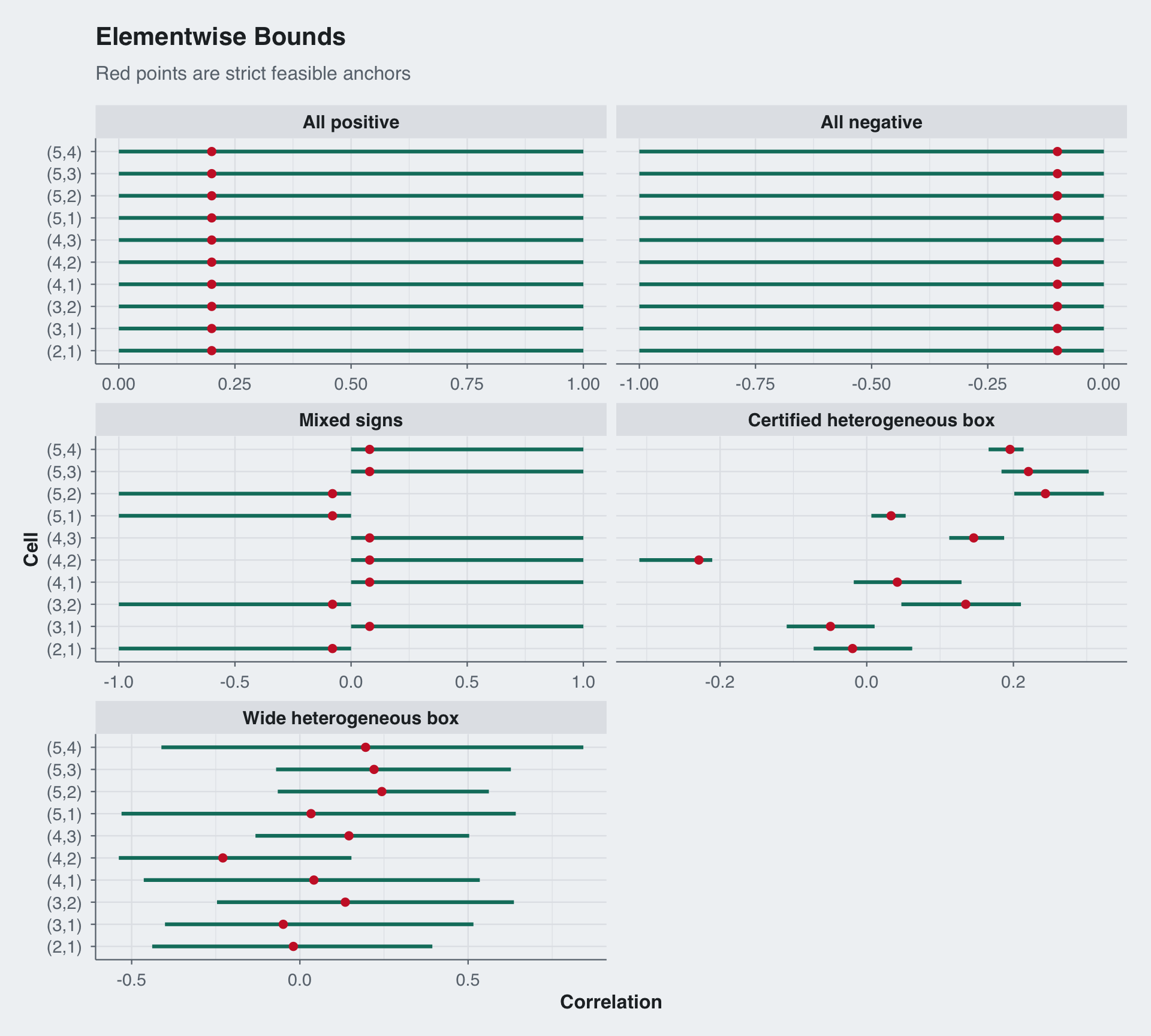
The first three boxes impose signs only. The two heterogeneous boxes contain different lower and upper endpoints for all ten cells, including intervals that do not contain zero.

Code
bounds |>
  mutate(
    scenario_label = factor(scenario_labels[scenario],
                            levels = unname(scenario_labels)),
    cell = sprintf("(%d,%d)", row, col)
  ) |>
  ggplot(aes(y = cell)) +
  geom_linerange(aes(xmin = lower, xmax = upper),
                 linewidth = 1.1, color = blog_colors$teal) +
  geom_point(aes(x = anchor), color = blog_colors$red, size = 2) +
  facet_wrap(~scenario_label, scales = "free_x", ncol = 2) +
  theme_blog() +
  labs(x = "Correlation", y = "Cell",
       title = "Elementwise Bounds",
       subtitle = "Red points are strict feasible anchors")
Figure 2: Bounds and strict feasible anchors used in the five experiments. The certified heterogeneous intervals lie wholly inside the elliptope; the wide heterogeneous box has non-PD corners.

7.2 A Numerical Cross-Check

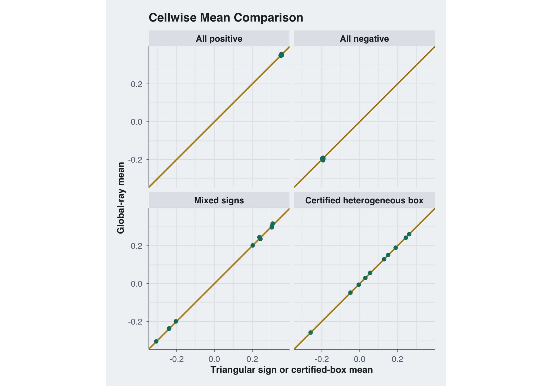
The derivations imply that the triangular sign map and global ray target the same bounded LKJ distribution in the first three scenarios. They likewise imply that the direct logistic and global ray have the same target for the certified heterogeneous box. The simulations provide a separate numerical check: across the 40 matched cell comparisons, the largest sample-mean difference is 0.010.

Code
ggplot(parity, aes(x = reference_mean, y = ray_mean)) +
  geom_abline(slope = 1, intercept = 0,
              color = blog_colors$gold, linewidth = 0.9) +
  geom_errorbar(aes(ymin = ray_mean - 2 * ray_mcse,
                    ymax = ray_mean + 2 * ray_mcse),
                width = 0, color = blog_colors$blue, alpha = 0.75) +
  geom_errorbar(aes(xmin = reference_mean - 2 * reference_mcse,
                    xmax = reference_mean + 2 * reference_mcse),
                orientation = "y", width = 0,
                color = blog_colors$blue, alpha = 0.75) +
  geom_point(color = blog_colors$teal, size = 2) +
  facet_wrap(~scenario_label) +
  coord_equal() +
  theme_blog() +
  labs(x = "Triangular sign or certified-box mean",
       y = "Global-ray mean",
       title = "Cellwise Mean Comparison")
Figure 3: Sample means from independent parameterizations of the same bounded LKJ targets. Error bars are two Monte Carlo standard errors; the diagonal is the equality line.

The largest difference is 2.50 combined Monte Carlo standard errors. Across the 5th, 50th, and 95th percentiles, the largest absolute quantile difference is 0.020. These are marginal implementation checks; they do not test the complete joint distribution or prove either Jacobian.

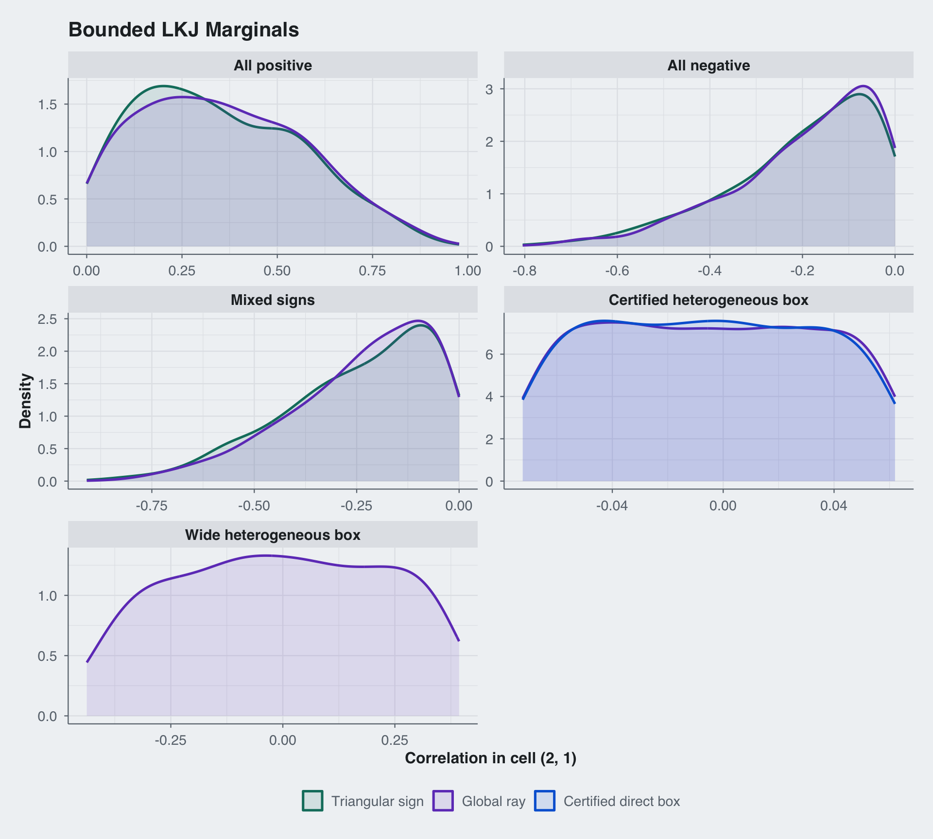
The next figure compares selected-cell marginals.

Code
ggplot(selected, aes(x = value, color = model_label, fill = model_label)) +
  geom_density(alpha = 0.12, linewidth = 0.9, adjust = 1.4) +
  facet_wrap(~scenario_label, scales = "free", ncol = 2) +
  scale_color_manual(values = c(
    "Triangular sign" = blog_colors$teal,
    "Global ray" = blog_colors$purple,
    "Certified direct box" = blog_colors$blue
  )) +
  scale_fill_manual(values = c(
    "Triangular sign" = blog_colors$teal,
    "Global ray" = blog_colors$purple,
    "Certified direct box" = blog_colors$blue
  )) +
  theme_blog() +
  theme(legend.position = "bottom") +
  labs(x = "Correlation in cell (2, 1)", y = "Density",
       color = NULL, fill = NULL,
       title = "Bounded LKJ Marginals")
Figure 4: Marginal draws for the first lower-triangular cell, Omega[2,1], under each pair of transforms.

7.3 Feasibility and HMC Performance in These Runs

Across the 54,000 retained matrices, the checks recorded no bound violations. The smallest sampled eigenvalue was positive in every fit, and there were no maximum-treedepth hits. Every sampled raw coordinate, including direction_raw and radius_raw, and every reported off-diagonal correlation had \(\widehat R<1.004\). The triangular sign map had no divergences in these runs. The global ray had one divergence in the mixed-sign case. A single divergent transition does not identify its cause; the piecewise boundary is one possible mechanism.

Code
diagnostics |>
  transmute(
    Scenario = scenario_label,
    Transform = model_label,
    Divergences = divergences,
    `Min bulk ESS` = round(pmin(min_bulk_ess, min_parameter_bulk_ess)),
    `Min corr ESS / 1k leapfrog steps` = round(ess_per_1000_gradients, 1),
    `Min E-BFMI` = round(min_ebfmi, 2),
    `Max R-hat` = round(pmax(max_rhat, max_parameter_rhat), 3),
    `PD boundary (%)` = ifelse(
      is.na(pd_boundary_fraction),
      "--",
      sprintf("%.1f", 100 * pd_boundary_fraction)
    ),
    `Time (s)` = round(seconds, 2),
    `Min eigenvalue` = signif(min_eigenvalue, 3)
  ) |>
  knitr::kable(align = c("l", "l", rep("r", 8)))
Table 2
Scenario Transform Divergences Min bulk ESS Min corr ESS / 1k leapfrog steps Min E-BFMI Max R-hat PD boundary (%) Time (s) Min eigenvalue
All positive Triangular sign 0 3877 59.7 0.87 1.002 0.27 0.002950
All positive Global ray 0 3049 5.7 0.78 1.001 59.4 1.19 0.000582
All negative Triangular sign 0 5492 122.7 0.81 1.002 0.15 0.000375
All negative Global ray 0 1877 1.3 0.78 1.003 42.9 3.17 0.001600
Mixed signs Triangular sign 0 4585 103.2 0.91 1.001 0.14 0.003020
Mixed signs Global ray 1 1900 1.3 0.71 1.003 66.2 2.65 0.002780
Certified heterogeneous box Certified direct box 0 8040 187.0 0.83 1.004 0.15 0.417000
Certified heterogeneous box Global ray 0 2505 3.4 0.71 1.001 0.0 1.62 0.421000
Wide heterogeneous box Global ray 0 3299 7.1 0.82 1.001 4.5 1.08 0.003540

The global construction was less efficient in these runs. It needs an eigendecomposition at every log-density evaluation, carries one auxiliary radial parameter, and uses the piecewise ray limit. Its minimum bulk ESS over the ten reported correlation cells per 1,000 recorded leapfrog steps was between 1.3 and 7.1, versus 59.7–122.7 for the triangular sign map and 187.0 for the certified direct box. The positive-definite boundary was active for 4.5% of the wide-box draws and was not active in the retained draws from the spectrally certified box.

8. What to Use

For an all-positive, all-negative, or prespecified mixed-sign pattern, I would start with the triangular sign transform. The formulas and row-wise inverse in Section 3 give a smooth bijection onto the interior of the signed elliptope. In exact arithmetic, every finite unconstrained state therefore produces a positive-definite correlation matrix with the requested signs, and every matrix in that constrained interior is represented. The calculation is triangular, with no eigendecomposition, auxiliary radial variable, or minimum over competing boundary distances.

The numerical comparison is consistent with that preference. In the three \(K=5\) sign experiments, the triangular map produced no divergences and achieved 59.7–122.7 minimum bulk ESS over the ten correlation cells per 1,000 recorded leapfrog steps. The global ray achieved 1.3–5.7 on the same targets and had one divergence in the mixed-sign case. These runs do not establish a general performance ordering. Coverage instead follows from the inverse maps in Sections 3 and 4: both maps represent the same sign-constrained interiors. The triangular construction is therefore my default for sign-only models.

An exact fixed value specifies a magnitude, not merely a sign. The affine triangular transform handles an individual row whenever the Schur-complement condition in Section 5 holds; if the predecessor block is fixed, that condition can be checked in advance. For a general pattern, however, the sequential construction can encounter internal prefix boundaries. Given a strict anchor, the reduced global ray avoids those prefix failures because it holds the fixed cells constant while exploring the feasible slice.

The other constructions handle positive-width finite intervals that the sign transform does not express. A cell-specific cap such as \(0<\rho_{ij}<u_{ij}<1\), or a finite interval \(\ell_{ij}<\rho_{ij}<u_{ij}\), is more than a sign constraint. If the entire resulting box can be certified positive definite, independent logits give the simpler smooth parameterization. Otherwise, if a strict anchor is available, the global ray covers the interior of the box–elliptope intersection at the cost of piecewise geometry and an eigendecomposition at every density evaluation.

One final qualification concerns \(\eta\). Everything here treats the LKJ shape as fixed. For a bounded region or affine equality slice \(\mathcal A\), the relevant normalizing integral is

\[Z_{\mathcal A}(\eta) =\int_{\mathcal A}\det(\Omega)^{\eta-1}\,d\mu_{\mathcal A}(\Omega),\]

where \(\mu_{\mathcal A}\) is Lebesgue measure on the remaining free correlations. If \(\eta\) is inferred, \(Z_{\mathcal A}(\eta)\) generally depends on \(\eta\) and cannot be dropped unless it is shown to be constant for the particular slice. The determinant kernel and change-of-variables Jacobian alone are sufficient here because \(\eta\) is fixed.

Reproducibility

The main benchmark is in benchmark_bounds.R; the exact-value rejection check is in benchmark_fixed_values.R. The downloadable tri-sign, global-ray, and certified-box Stan programs are in the same published directory. The global-ray program accepts both positive-width intervals and exact cells; the other two programs retain their narrower interfaces. Each script checks its applicable bounds or fixed values and sampled eigenvalues, and records the sampler diagnostics reported above.

The published results are the main diagnostics, cell summaries, scenario bounds, and plotted draw subset, together with the fixed-value diagnostics and comparison. Run settings and source checksums are recorded in bounds-run-settings.csv, bounds-source-hashes.csv, fixed-values-run-settings.csv, and fixed-values-source-hashes.csv.

Appendix: Stan Implementations

tri-sign-corr-bounds.stan
/*
  Smooth triangular transform for prescribed correlation signs.

  Every off-diagonal cell is either positive, with bounds [0, 1], or
  negative, with bounds [-1, 0].  In Cholesky row i, let B be the leading
  Cholesky block and c the ordinary correlations with earlier variables.
  The transform creates a vector x in the requested orthant, solves

      w = B^{-1} x,

  and applies the modified stereographic hemisphere map

      z = sqrt(w'w + 2) / (w'w + 1) * w,
      L[i,i] = 1 / (w'w + 1).

  Because c = B z is a positive scalar multiple of x, every requested sign
  is exact and every raw value produces a positive-definite correlation
  matrix.  The B and B^{-1} determinants cancel in the raw-to-c Jacobian.
*/

functions {
  tuple(matrix, real) corr_cholesky_sign_jacobian(
      int K,
      vector raw,
      matrix corr_lower,
      matrix corr_upper) {
    matrix[K, K] L = rep_matrix(0.0, K, K);
    int raw_pos = 1;
    real log_det = 0.0;
    real input_scale = 2.0 * K;

    L[1, 1] = 1.0;

    for (i in 2:K) {
      int d = i - 1;
      vector[d] x;
      matrix[d, d] previous_cholesky = L[1:d, 1:d];

      for (j in 1:d) {
        real raw_ij = raw[raw_pos + j - 1];
        real magnitude = log1p_exp(raw_ij) / input_scale;
        real sign_ij = corr_lower[i, j] == 0.0 ? 1.0 : -1.0;

        x[j] = sign_ij * magnitude;
        jacobian += log_inv_logit(raw_ij) - log(input_scale);
      }

      {
        vector[d] w = mdivide_left_tri_low(previous_cholesky, x);
        real t = dot_self(w);
        real scale = sqrt(t + 2.0) / (t + 1.0);

        L[i, 1:d] = (scale * w)';
        L[i, i] = 1.0 / (t + 1.0);
        log_det += 2.0 * log(L[i, i]);

        // Exact determinant of w -> scale(t) * w.  The constant log(2)
        // is retained even though it could be dropped from the target.
        jacobian += log(2.0)
                    + 0.5 * (d - 2.0) * log(t + 2.0)
                    - (d + 1.0) * log1p(t);
      }

      raw_pos += d;
    }

    if (raw_pos != num_elements(raw) + 1) {
      reject("Sign transform consumed ", raw_pos - 1,
             " raw values but received ", num_elements(raw), ".");
    }

    return (L, log_det);
  }
}

data {
  int<lower=2> K;
  real<lower=0> eta;
  matrix[K, K] corr_lower;
  matrix[K, K] corr_upper;
  real<lower=0> validation_tolerance;
}

transformed data {
  if (!(eta > 0.0)) {
    reject("The LKJ shape eta must be strictly positive; received ", eta,
           ".");
  }

  for (i in 1:K) {
    if (abs(corr_lower[i, i] - 1.0) > validation_tolerance
        || abs(corr_upper[i, i] - 1.0) > validation_tolerance) {
      reject("Both bound matrices must equal one on diagonal ", i, ".");
    }

    if (i > 1) {
      for (j in 1:(i - 1)) {
        real lo = corr_lower[i, j];
        real hi = corr_upper[i, j];
        int positive_sign = lo == 0.0 && hi == 1.0;
        int negative_sign = lo == -1.0 && hi == 0.0;

        if (abs(lo - corr_lower[j, i]) > validation_tolerance
            || abs(hi - corr_upper[j, i]) > validation_tolerance) {
          reject("Bounds are not symmetric at pair (", i, ",", j, ").");
        }
        if (!(positive_sign || negative_sign)) {
          reject("Pair (", i, ",", j,
                 ") must request [0,1] or [-1,0]; received [",
                 lo, ",", hi, "].");
        }
      }
    }
  }
}

parameters {
  vector[choose(K, 2)] raw;
}

transformed parameters {
  matrix[K, K] L_Omega;
  corr_matrix[K] Omega;
  real log_det_Omega;

  {
    tuple(matrix[K, K], real) result = corr_cholesky_sign_jacobian(
        K, raw, corr_lower, corr_upper);
    L_Omega = result.1;
    log_det_Omega = result.2;
    Omega = multiply_lower_tri_self_transpose(L_Omega);
  }
}

model {
  target += (eta - 1.0) * log_det_Omega;
}
global-ray-corr-bounds.stan
/*
  Globally feasible transform for arbitrary elementwise correlation bounds
  and exact fixed ordinary correlations.

  The feasible set is the intersection of the positive-definite correlation
  cone and an ordinary-correlation box.  Given a strictly interior anchor,
  every ray from that anchor remains feasible until it first reaches either a
  box face or the positive-definite boundary.  Cells whose lower and upper
  bounds are exactly equal are held fixed and omitted from the direction
  vector.  An auxiliary isotropic normal vector supplies a uniform direction
  on the sphere of the remaining free coordinates; its radius is independent
  of the resulting correlation matrix.

  The target is det(Omega)^(eta - 1) with respect to the remaining free
  ordinary off-diagonal correlations.
*/

functions {
  tuple(matrix, real, real, real, real) corr_global_ray_jacobian(
      vector direction_raw,
      real radius_raw,
      matrix corr_lower,
      matrix corr_upper,
      matrix anchor,
      matrix anchor_cholesky) {
    int K = rows(anchor);
    int D = num_elements(direction_raw);
    real direction_norm = sqrt(dot_self(direction_raw));
    vector[D] direction;
    matrix[K, K] direction_matrix = rep_matrix(0.0, K, K);
    real max_radius_box = positive_infinity();
    real max_radius_pd = positive_infinity();
    real max_radius;
    real radius_fraction = inv_logit(radius_raw);
    real radius;
    matrix[K, K] Omega;
    real log_det;
    int pos = 1;

    if (!(direction_norm > 0.0)) {
      reject("The auxiliary direction vector has zero norm.");
    }
    if (!(radius_fraction > 0.0 && radius_fraction < 1.0)) {
      reject("The radial inverse logit reached an endpoint; raw value=",
             radius_raw, ".");
    }

    direction = direction_raw / direction_norm;

    for (i in 2:K) {
      for (j in 1:(i - 1)) {
        if (corr_lower[i, j] != corr_upper[i, j]) {
          real component = direction[pos];
          real distance_to_face;

          direction_matrix[i, j] = component;
          direction_matrix[j, i] = component;

          if (component > 0.0) {
            distance_to_face = (corr_upper[i, j] - anchor[i, j])
                               / component;
            max_radius_box = fmin(max_radius_box, distance_to_face);
          } else if (component < 0.0) {
            distance_to_face = (corr_lower[i, j] - anchor[i, j])
                               / component;
            max_radius_box = fmin(max_radius_box, distance_to_face);
          }

          pos += 1;
        }
      }
    }

    if (pos != D + 1) {
      reject("Global-ray transform consumed ", pos - 1,
             " free direction values but received ", D, ".");
    }

    // C(t) = C0 + t*S is positive definite exactly while
    // I + t * L0^{-1} S L0^{-T} is positive definite.
    {
      matrix[K, K] left_solve = mdivide_left_tri_low(
          anchor_cholesky, direction_matrix);
      matrix[K, K] standardized_direction = mdivide_left_tri_low(
          anchor_cholesky, left_solve')';
      vector[K] eigenvalues = eigenvalues_sym(
          0.5 * (standardized_direction + standardized_direction'));
      real lambda_min = eigenvalues[1];

      if (lambda_min < 0.0) {
        max_radius_pd = -1.0 / lambda_min;
      }
      max_radius = fmin(max_radius_box, max_radius_pd);
    }

    if (!(max_radius > 0.0) || is_inf(max_radius)) {
      reject("The supplied anchor has no finite positive ray in this ",
             "direction; max_radius=", max_radius, ".");
    }

    radius = radius_fraction * max_radius;
    Omega = anchor + radius * direction_matrix;

    {
      matrix[K, K] L = cholesky_decompose(Omega);
      log_det = 2.0 * sum(log(diagonal(L)));
    }

    // In D dimensions, dc = radius^(D-1) d(radius) d(surface).
    // Normalizing an isotropic standard-normal auxiliary vector supplies
    // uniform surface measure, so only the ray and logistic terms remain.
    jacobian += (D - 1.0) * log(radius)
                + log(max_radius)
                + log_inv_logit(radius_raw)
                + log1m_inv_logit(radius_raw);

    return (Omega, log_det, max_radius, max_radius_box, max_radius_pd);
  }
}

data {
  // With only one free cell, at any K, the unit direction is the
  // discontinuous sign of one scalar; use a direct bounded logistic for
  // that one-dimensional special case.
  int<lower=3> K;
  real<lower=0> eta;
  int<lower=0, upper=choose(K, 2)> N_fixed;
  matrix[K, K] corr_lower;
  matrix[K, K] corr_upper;
  corr_matrix[K] anchor;
  real<lower=0> validation_tolerance;
}

transformed data {
  matrix[K, K] anchor_cholesky = cholesky_decompose(anchor);
  int fixed_count = 0;
  int D_free = choose(K, 2) - N_fixed;

  if (!(eta > 0.0)) {
    reject("The LKJ shape eta must be strictly positive; received ", eta,
           ".");
  }
  if (D_free < 2) {
    reject("The normalized-direction global-ray transform requires at least ",
           "two free correlations; received ", D_free, ".");
  }

  for (i in 1:K) {
    if (abs(corr_lower[i, i] - 1.0) > validation_tolerance
        || abs(corr_upper[i, i] - 1.0) > validation_tolerance) {
      reject("Both bound matrices must equal one on diagonal ", i, ".");
    }

    if (i > 1) {
      for (j in 1:(i - 1)) {
        real lo = corr_lower[i, j];
        real hi = corr_upper[i, j];

        if (abs(lo - corr_lower[j, i]) > validation_tolerance
            || abs(hi - corr_upper[j, i]) > validation_tolerance) {
          reject("Bounds are not symmetric at pair (", i, ",", j, ").");
        }
        if (lo < -1.0 || hi > 1.0 || lo > hi) {
          reject("Pair (", i, ",", j,
                 ") must have ordered bounds inside [-1,1]; got [",
                 lo, ",", hi, "].");
        }

        if (lo == hi) {
          fixed_count += 1;
          if (anchor[i, j] != lo) {
            reject("Anchor must equal the exact fixed value at pair (", i,
                   ",", j, "): anchor=", anchor[i, j],
                   ", fixed value=", lo, ".");
          }
        } else {
          if (!(anchor[i, j] > lo + validation_tolerance
                && anchor[i, j] < hi - validation_tolerance)) {
            reject("Anchor is not strictly inside the bounds at pair (", i,
                   ",", j, "): anchor=", anchor[i, j], ", bounds=[",
                   lo, ",", hi, "].");
          }
        }
      }
    }
  }

  if (fixed_count != N_fixed) {
    reject("N_fixed declares ", N_fixed, " exact cells, but the lower and ",
           "upper bound matrices contain ", fixed_count,
           " equal off-diagonal pairs.");
  }
}

parameters {
  vector[choose(K, 2) - N_fixed] direction_raw;
  real radius_raw;
}

transformed parameters {
  corr_matrix[K] Omega;
  real log_det_Omega;
  real max_radius;
  real max_radius_box;
  real max_radius_pd;
  real pd_boundary_active;

  {
    tuple(matrix[K, K], real, real, real, real) result
        = corr_global_ray_jacobian(
            direction_raw, radius_raw,
            corr_lower, corr_upper, anchor, anchor_cholesky);
    Omega = result.1;
    log_det_Omega = result.2;
    max_radius = result.3;
    max_radius_box = result.4;
    max_radius_pd = result.5;
    pd_boundary_active = max_radius_pd < max_radius_box ? 1.0 : 0.0;
  }
}

model {
  // The auxiliary radius integrates out independently; isotropy makes the
  // normalized direction uniform on the sphere.
  direction_raw ~ std_normal();
  target += (eta - 1.0) * log_det_Omega;
}
direct-certified-box-corr.stan
/*
  Direct ordinary-correlation transform for a box certified to lie entirely
  inside the positive-definite correlation cone.

  This model deliberately performs no feasibility look-ahead.  It is valid
  only when the supplied box has been certified externally (for example with
  a spectral-norm/Weyl bound around a positive-definite anchor).
*/

data {
  int<lower=2> K;
  real<lower=0> eta;
  matrix[K, K] corr_lower;
  matrix[K, K] corr_upper;
  real<lower=0> validation_tolerance;
}

transformed data {
  if (!(eta > 0.0)) {
    reject("The LKJ shape eta must be strictly positive; received ", eta,
           ".");
  }

  for (i in 1:K) {
    if (abs(corr_lower[i, i] - 1.0) > validation_tolerance
        || abs(corr_upper[i, i] - 1.0) > validation_tolerance) {
      reject("Both bound matrices must equal one on diagonal ", i, ".");
    }

    if (i > 1) {
      for (j in 1:(i - 1)) {
        real lo = corr_lower[i, j];
        real hi = corr_upper[i, j];

        if (abs(lo - corr_lower[j, i]) > validation_tolerance
            || abs(hi - corr_upper[j, i]) > validation_tolerance) {
          reject("Bounds are not symmetric at pair (", i, ",", j, ").");
        }
        if (lo < -1.0 || hi > 1.0 || !(lo < hi)) {
          reject("Pair (", i, ",", j,
                 ") must have positive-width bounds inside [-1,1]; got [",
                 lo, ",", hi, "].");
        }
      }
    }
  }
}

parameters {
  vector[choose(K, 2)] raw;
}

transformed parameters {
  corr_matrix[K] Omega;
  real log_det_Omega;

  {
    matrix[K, K] work = identity_matrix(K);
    int pos = 1;

    for (i in 2:K) {
      for (j in 1:(i - 1)) {
        real value = lower_upper_bound_jacobian(
            raw[pos], corr_lower[i, j], corr_upper[i, j]);
        work[i, j] = value;
        work[j, i] = value;
        pos += 1;
      }
    }

    Omega = work;
    log_det_Omega = log_determinant_spd(Omega);
  }
}

model {
  target += (eta - 1.0) * log_det_Omega;
}

References

Axen, Seth. 2023. Comment on “Covariance Conditioned on Undirected Graph”. TuringLang/Turing.jl GitHub discussion #2067. https://github.com/TuringLang/Turing.jl/discussions/2067#discussioncomment-7023577.
Carpenter, Bob, Andrew Gelman, Matthew D. Hoffman, et al. 2017. “Stan: A Probabilistic Programming Language.” Journal of Statistical Software 76 (1): 1–32. https://doi.org/10.18637/jss.v076.i01.
Horn, Roger A., and Charles R. Johnson. 2013. Matrix Analysis. 2nd ed. Cambridge University Press. https://doi.org/10.1017/CBO9781139020411.
Lewandowski, Daniel, Dorota Kurowicka, and Harry Joe. 2009. “Generating Random Correlation Matrices Based on Vines and Extended Onion Method.” Journal of Multivariate Analysis 100 (9): 1989–2001. https://doi.org/10.1016/j.jmva.2009.04.008.
Pinkney, Sean. 2024. A Short Note on a Flexible Cholesky Parameterization of Correlation Matrices. https://arxiv.org/abs/2405.07286.
Pinkney, Sean. 2025. Updated Cholesky Corr Parameterization Testing. Stan Discourse thread. https://discourse.mc-stan.org/t/updated-cholesky-corr-parameterization-testing/38827.
Sylvester, J. J. 1852. XIX. A Demonstration of the Theorem That Every Homogeneous Quadratic Polynomial Is Reducible by Real Orthogonal Substitutions to the Form of a Sum of Positive and Negative Squares.” The London, Edinburgh, and Dublin Philosophical Magazine and Journal of Science 4 (23): 138–42. https://doi.org/10.1080/14786445208647087.